arcgis-212244
Inspecting mapped polygons and attributes
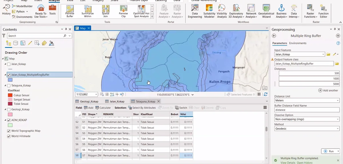
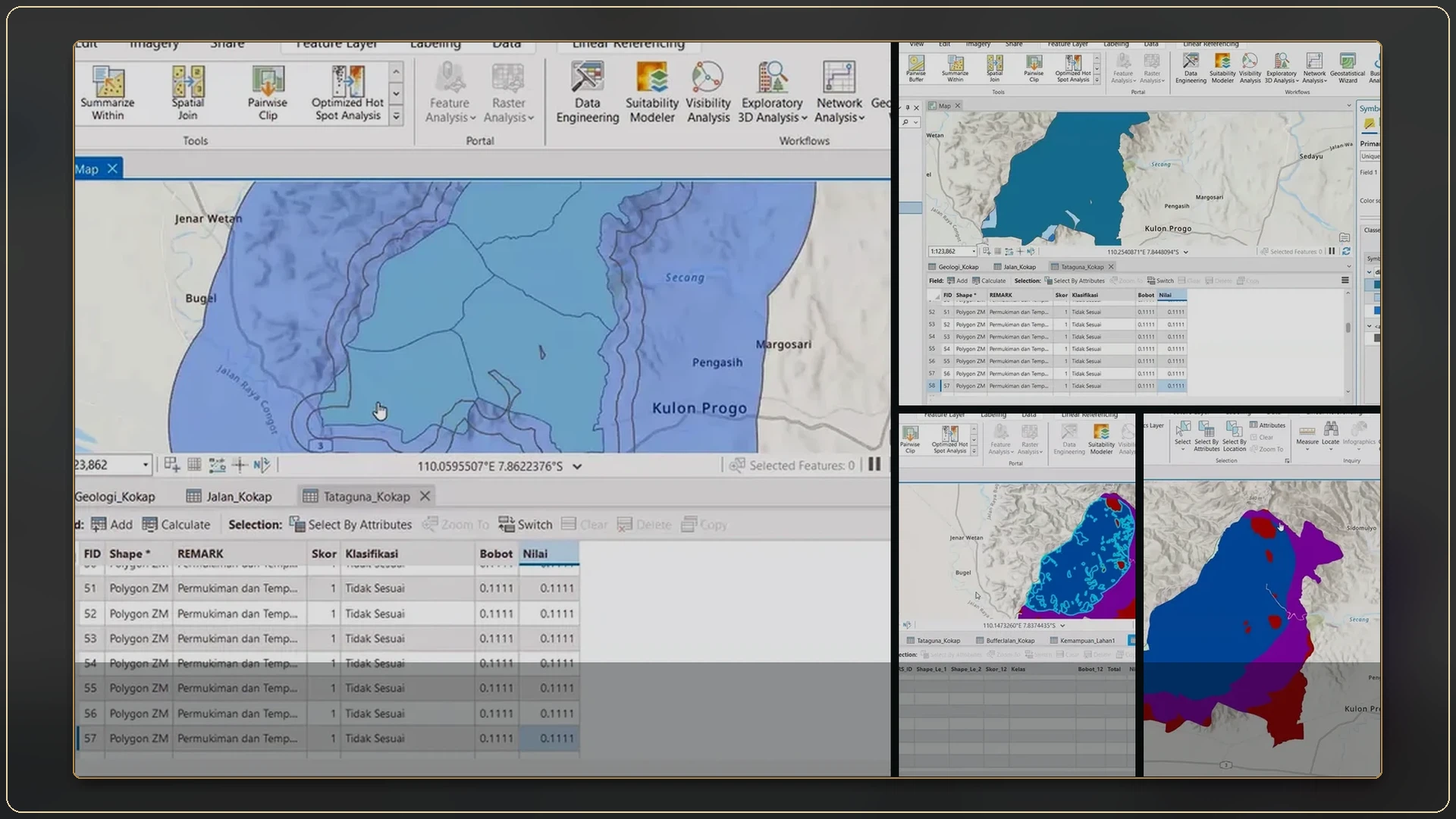
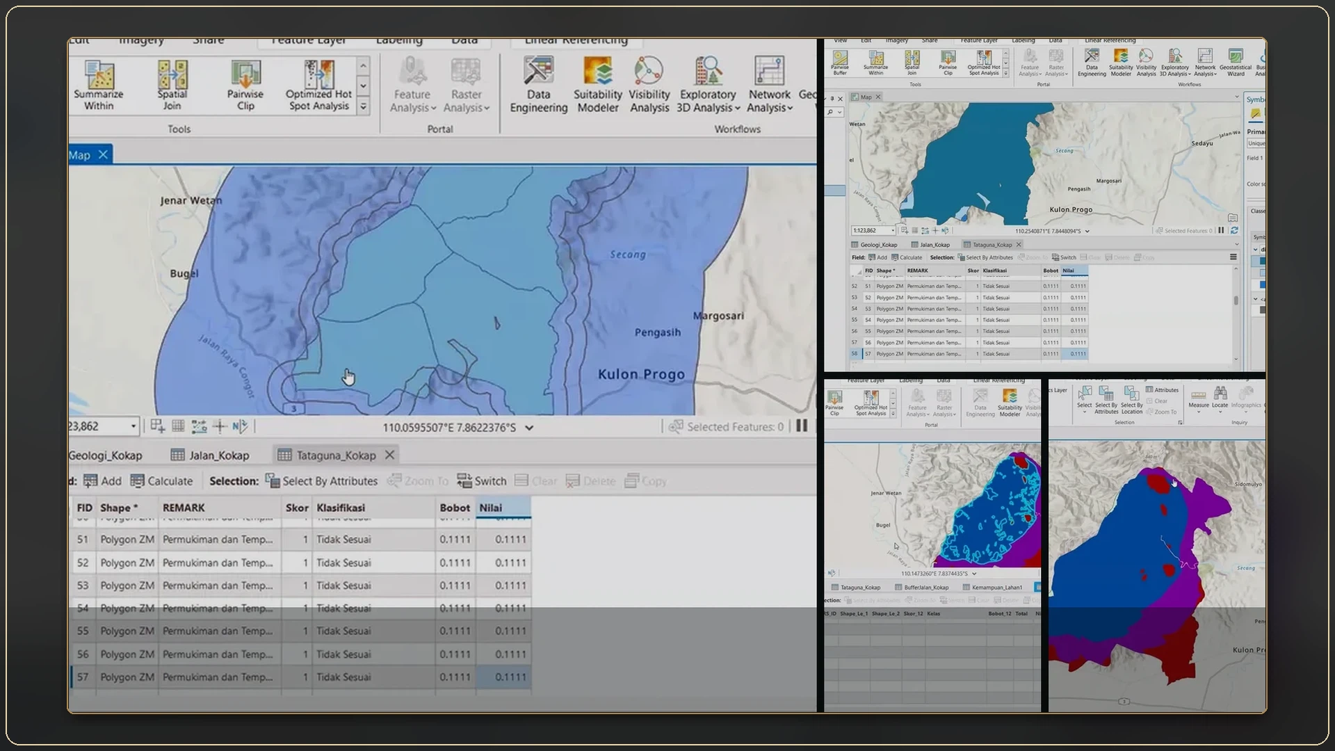
Stage 01 of the ArcGIS Pro sequence: the map, layer list and attribute table are reviewed together to confirm polygon identity, field values and layer order before symbol assignment.
Software Documentation
All 127 records are shown below, grouped by album.
ALBUM
10 records
Stage 01 of the ArcGIS Pro sequence: the map, layer list and attribute table are reviewed together to confirm polygon identity, field values and layer order before symbol assignment.
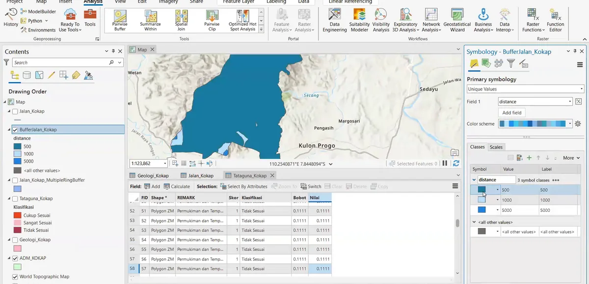
Stage 02 of the ArcGIS Pro sequence: a selected polygon layer is symbolised from its geological attribute, with fill colour and class settings adjusted in the Symbology pane.
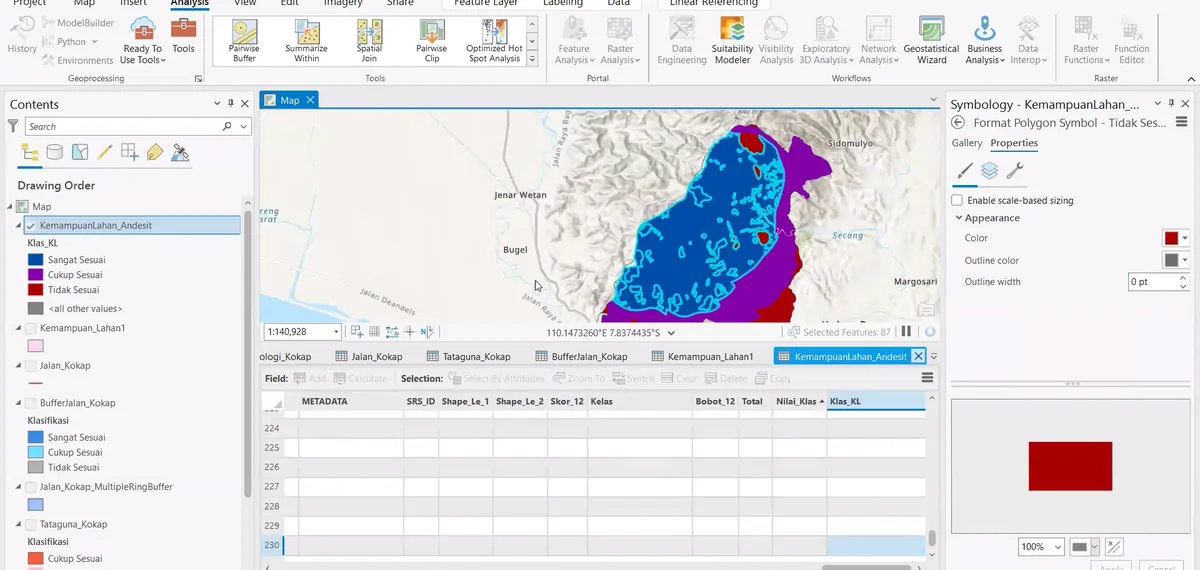
Stage 03 of the ArcGIS Pro sequence: colour-coded polygons are compared with the attribute table to verify that each mapped unit is assigned to the intended class.
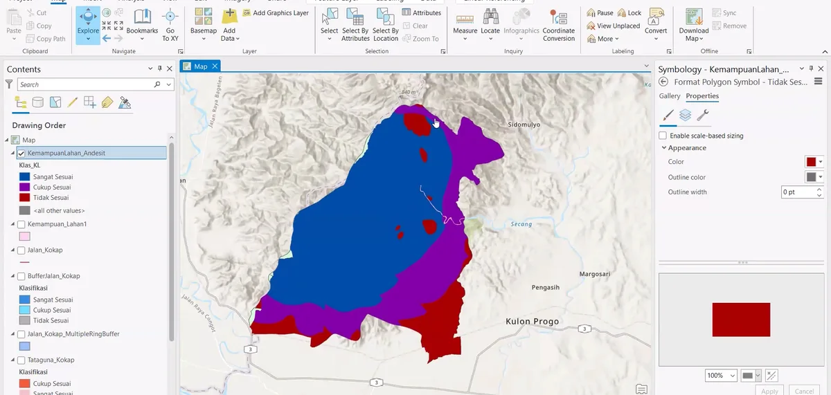
Stage 04 of the ArcGIS Pro sequence: symbol properties are adjusted for individual geological classes while the mapped polygons remain visible against the terrain base.
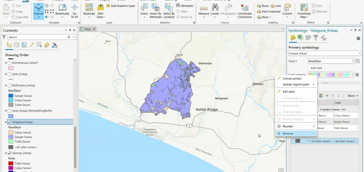
Stage 05 of the ArcGIS Pro sequence: geological features are selected and inspected against the basemap to confirm their extent, identity and spatial relationship with neighbouring units.
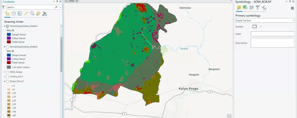
Stage 06 of the ArcGIS Pro sequence: the mapped units are displayed with a revised colour hierarchy and contrasting boundaries to improve separation between formations.
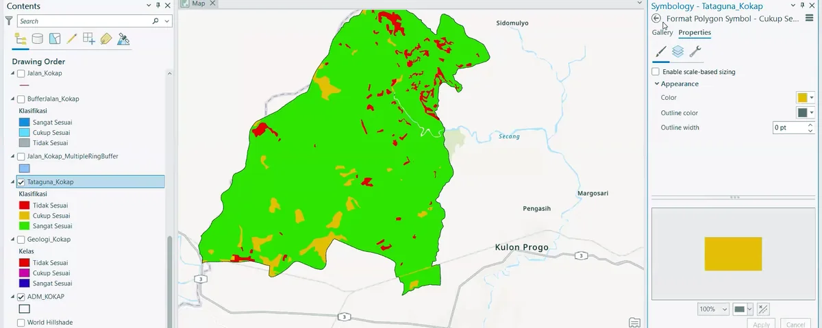
Stage 07 of the ArcGIS Pro sequence: formation polygons, linear features and point observations are inspected together to locate boundary gaps, overlaps or features assigned to the wrong unit.
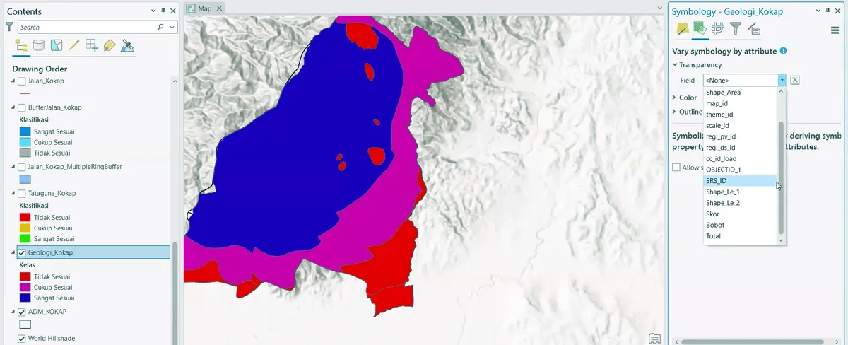
Stage 08 of the ArcGIS Pro sequence: alternative colour classifications are compared on the same mapped extent to confirm that the final legend preserves the intended unit relationships.
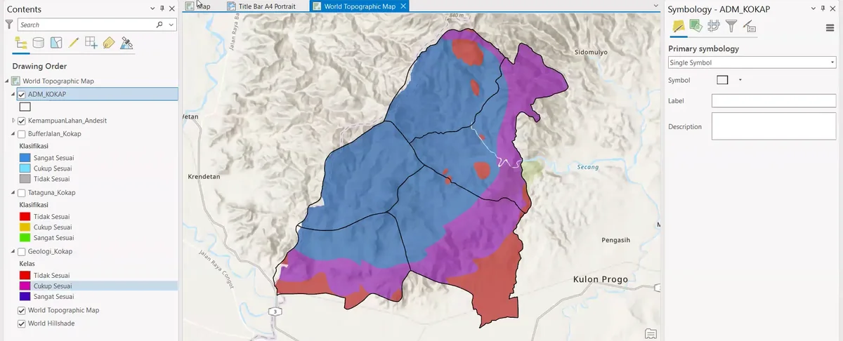
Stage 09 of the ArcGIS Pro sequence: the geological map is arranged with its thematic layers, drainage and supporting map elements in a publication layout.
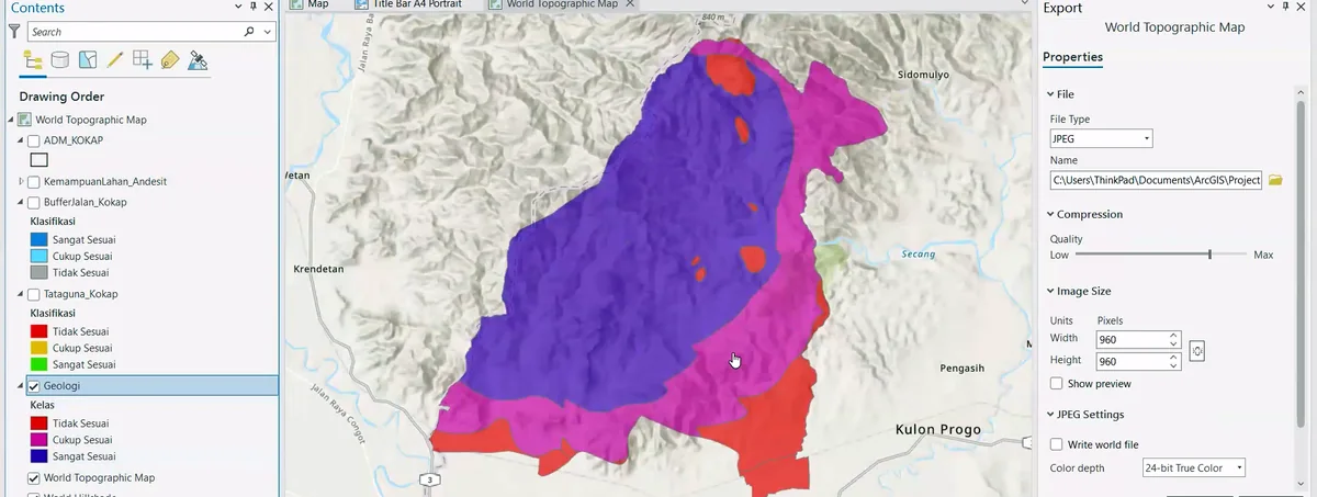
Stage 10 of the ArcGIS Pro sequence: the completed map and legend are reviewed at output scale, with the final symbology and page composition visible together.
ALBUM
2 records
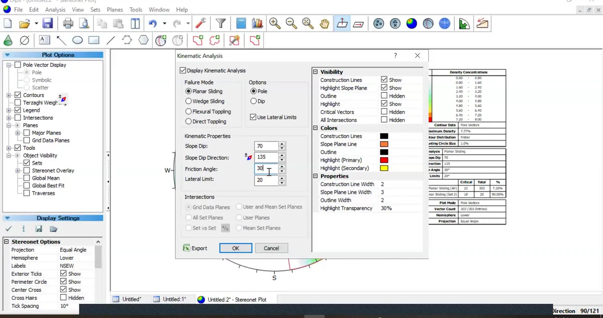
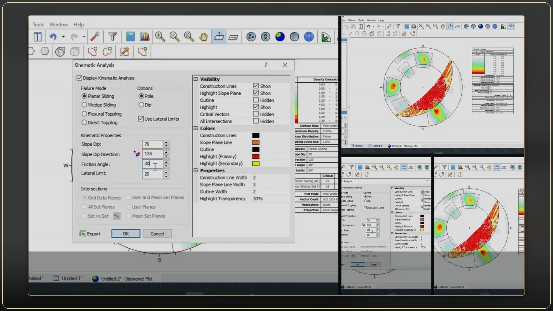
Stage 01 of the Rocscience Dips sequence: orientation data, slope attitude, friction angle and kinematic-analysis settings are entered before the stereonet is evaluated.
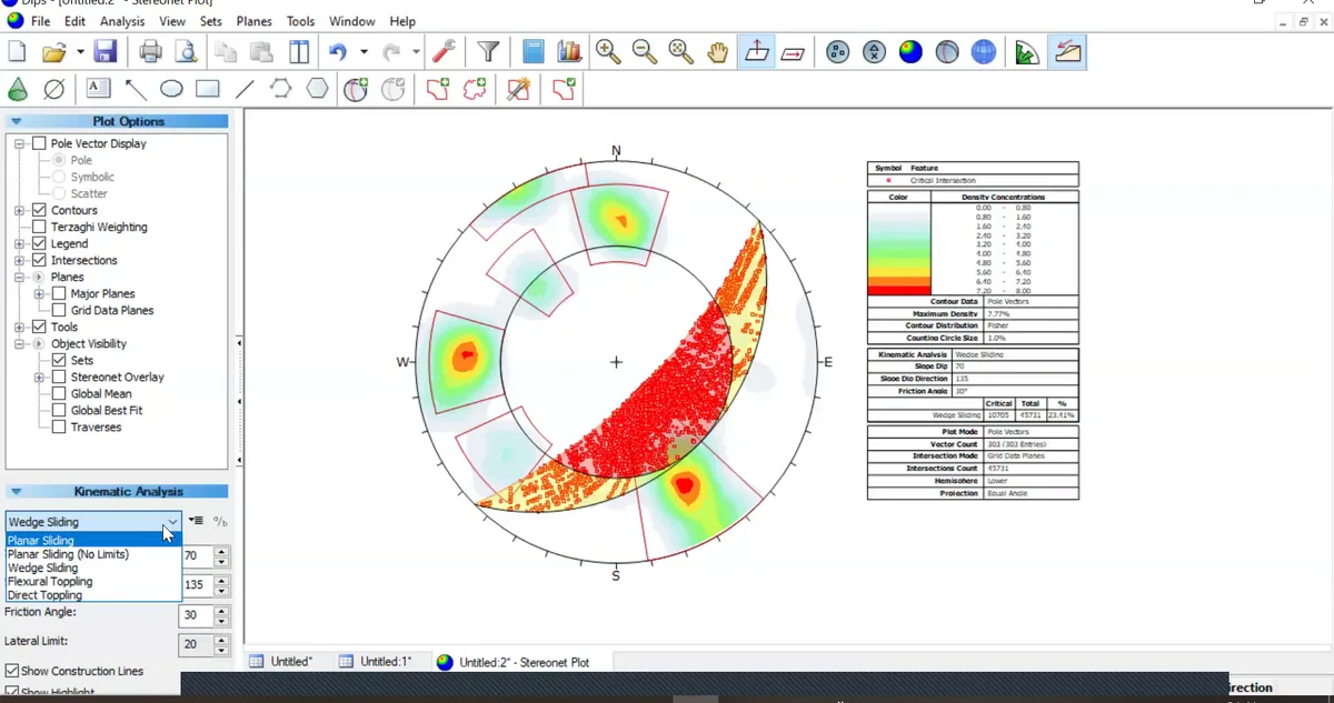
Stage 02 of the Rocscience Dips sequence: pole-density clusters, mean discontinuity sets and the critical kinematic zone are reviewed on the stereonet to identify structurally admissible failure directions.
ALBUM
5 records
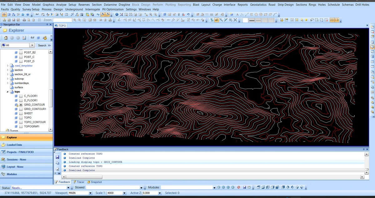
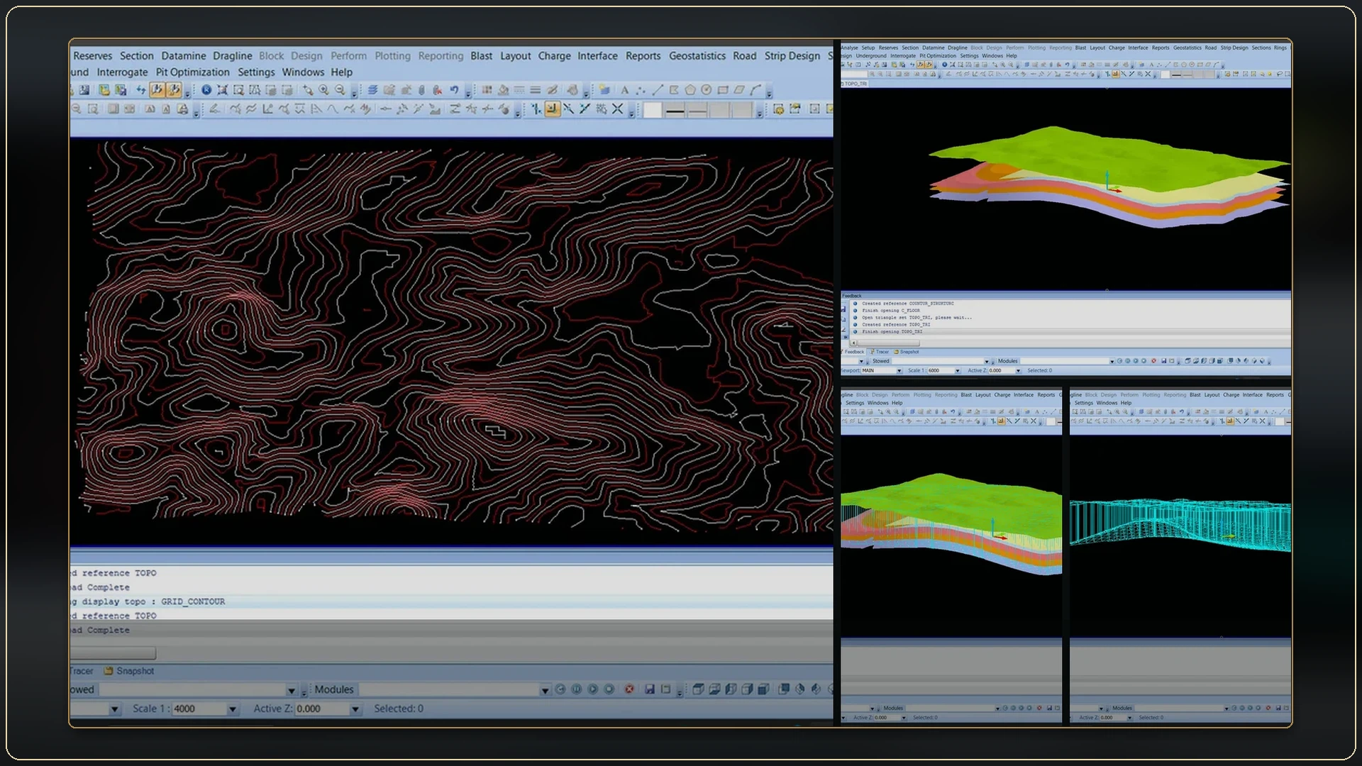
The TOPO view displays the contour network used to establish elevation control and the upper boundary of the seam model.
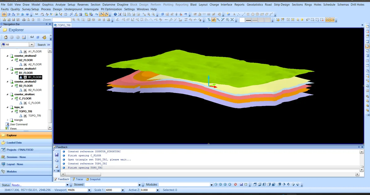
Topography and the interpreted floors of Seams A2, B1, B2 and C are displayed together to inspect stratigraphic order and lateral geometry.
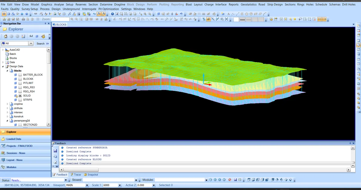
Vertical cells are generated between the model boundaries, converting the surface interpretation into a spatial framework that can carry geological attributes.
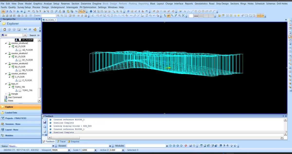
The wireframe exposes cell arrangement, lateral extent and vertical conformity to the model boundaries.
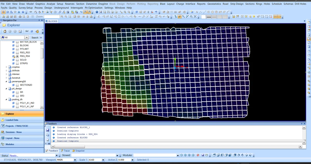
The plan view shows colour-separated cell domains alongside the controlling polygon objects.
ALBUM
16 records
Stage 01 of the Micromine Origin sequence: the Micromine Origin project view displays the active geological objects at the 3d project scene and data loading stage.
Stage 02 of the Micromine Origin sequence: drillholes and their coded intervals are displayed in three dimensions to confirm collar positions, trace orientation and the spatial distribution of geological control.
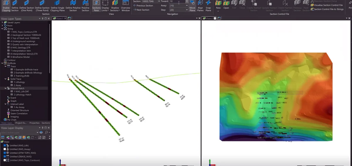
Stage 03 of the Micromine Origin sequence: interpretation strings are reviewed across the available sections, preserving the boundaries used to construct the geological domain.
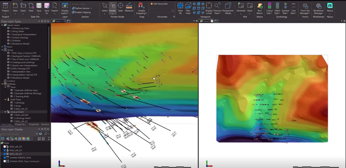
Stage 04 of the Micromine Origin sequence: the interpreted boundary is converted into a triangulated surface and inspected for continuity, edge behaviour and local geometric artefacts.
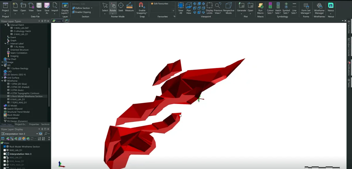
Stage 05 of the Micromine Origin sequence: bounding surfaces are joined into a closed geological solid that represents the interpreted three-dimensional domain.
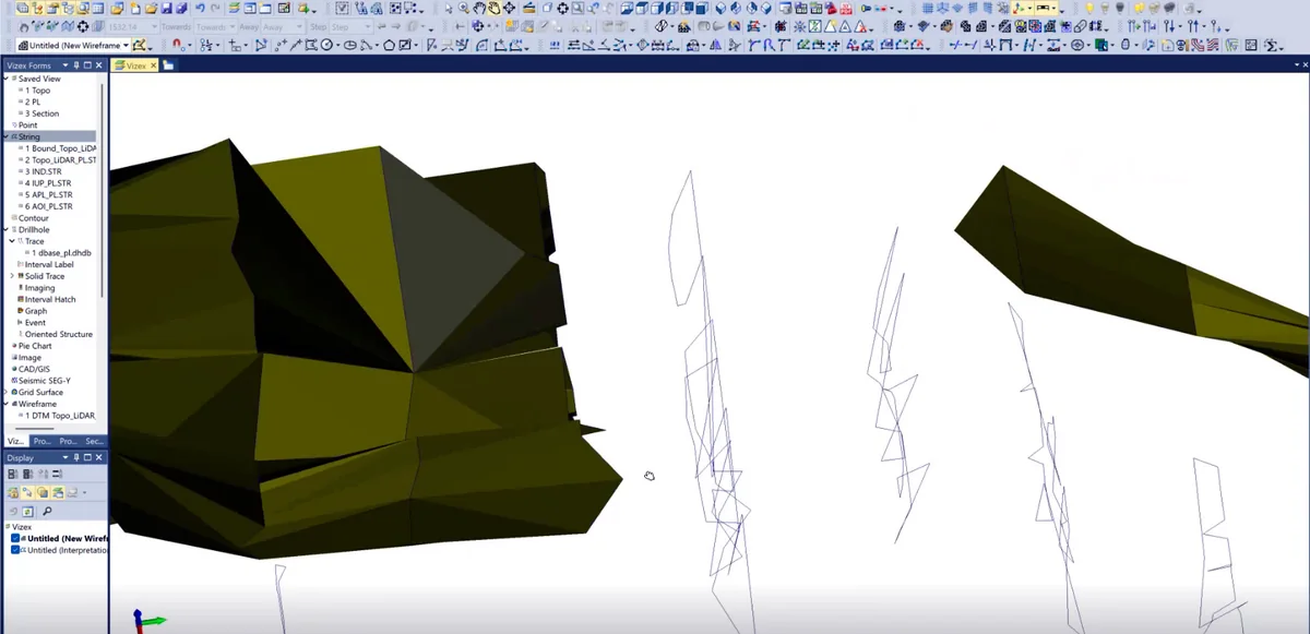
Stage 06 of the Micromine Origin sequence: a sectional cut exposes the internal relationship between the model, interpreted boundaries and the available geological control.
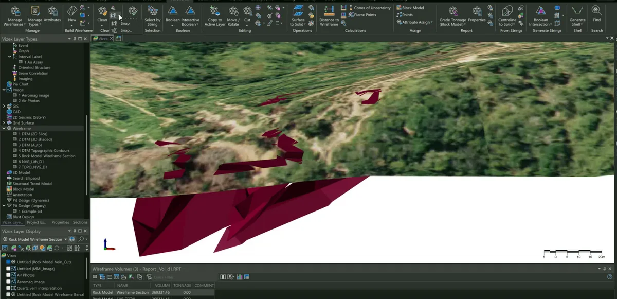
Stage 07 of the Micromine Origin sequence: bounding surfaces are joined into a closed geological solid that represents the interpreted three-dimensional domain.
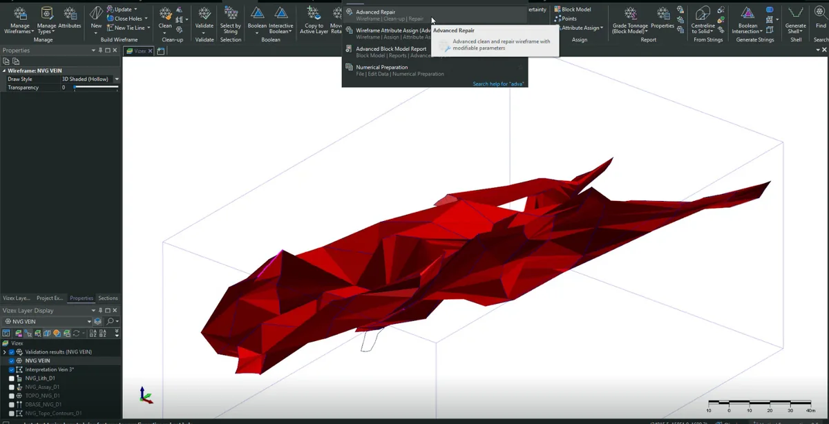
Stage 08 of the Micromine Origin sequence: the geological interpretation is placed against the topographic surface to verify its position, extent and relationship with the ground surface.
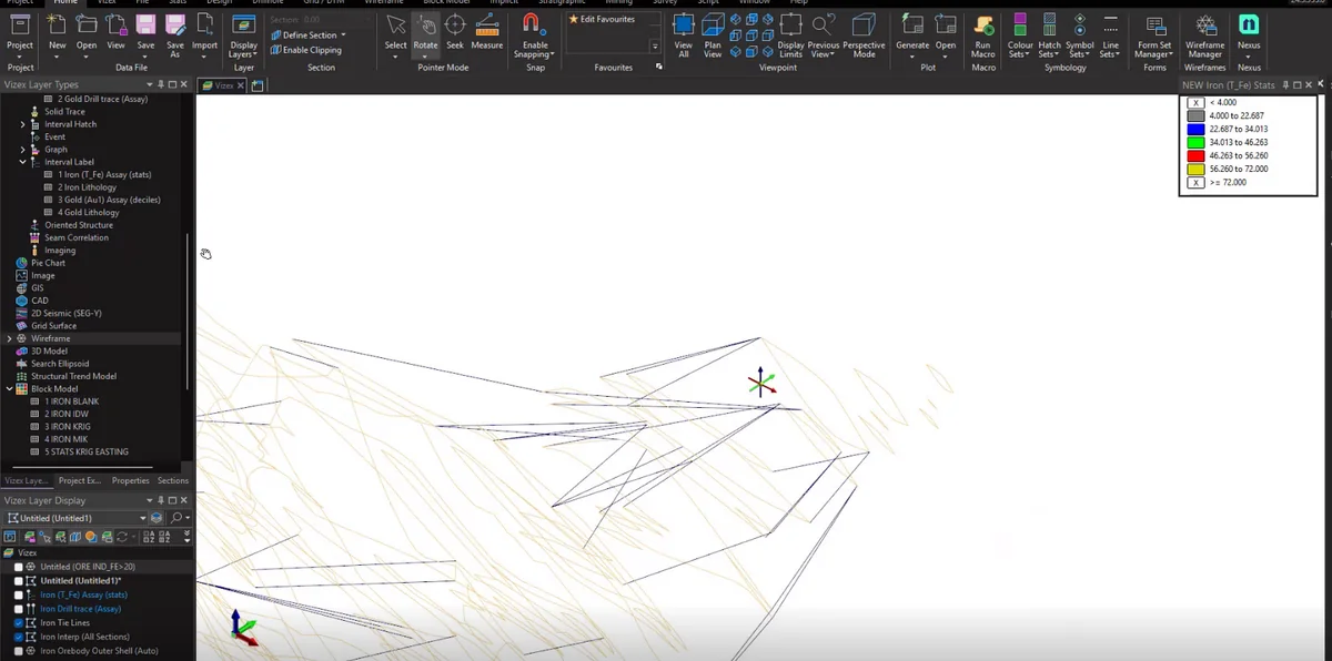
Stage 09 of the Micromine Origin sequence: a regular three-dimensional cell framework is generated across the interpreted domain, providing the structure required to store geological or quantitative attributes.
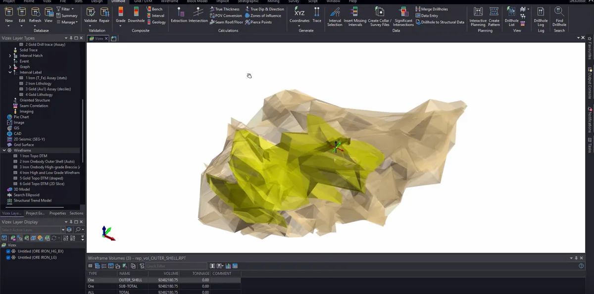
Stage 10 of the Micromine Origin sequence: the model is coloured by an assigned attribute so that spatial changes and domain boundaries can be inspected directly.
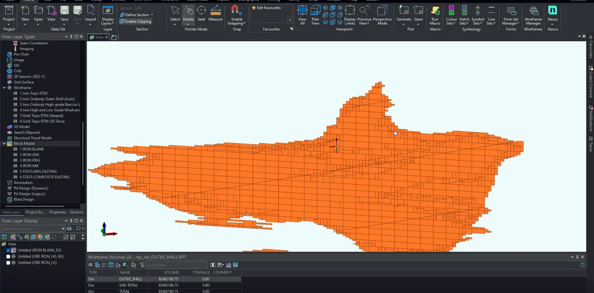
Stage 11 of the Micromine Origin sequence: a sectional cut exposes the internal relationship between the model, interpreted boundaries and the available geological control.
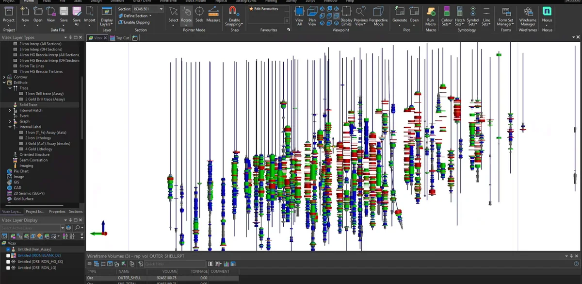
Stage 12 of the Micromine Origin sequence: the interpreted surfaces, solids or model cells are isolated and compared to check continuity, boundary conformity and internal consistency.
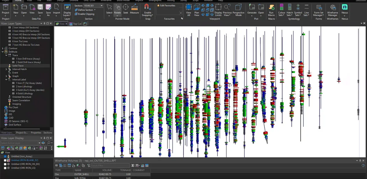
Stage 13 of the Micromine Origin sequence: the interpreted surfaces, solids or model cells are isolated and compared to check continuity, boundary conformity and internal consistency.
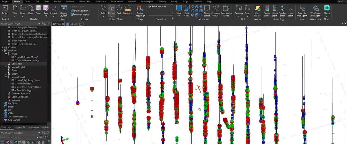
Stage 14 of the Micromine Origin sequence: the interpreted surfaces, solids or model cells are isolated and compared to check continuity, boundary conformity and internal consistency.
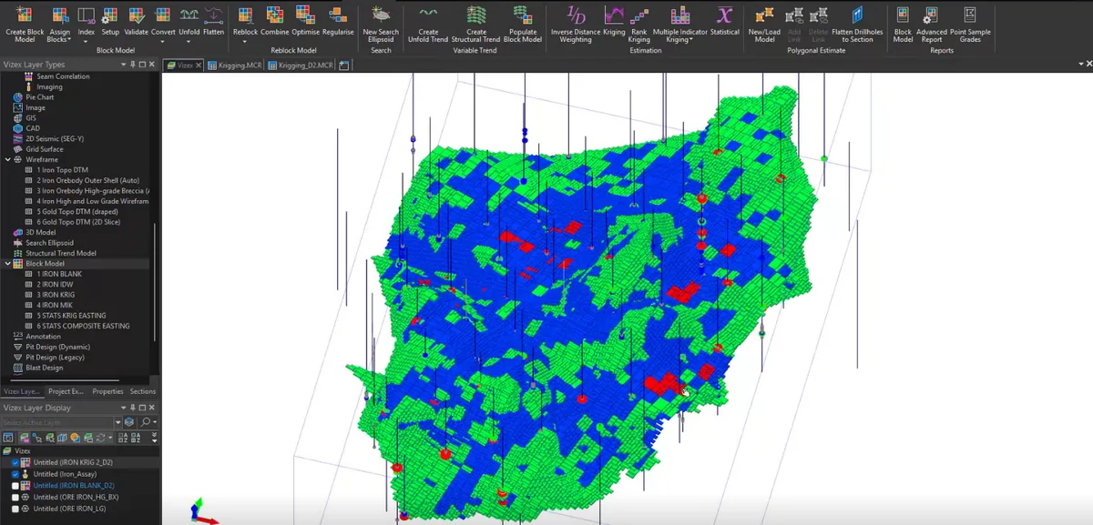
Stage 15 of the Micromine Origin sequence: the principal model components are assembled in a final three-dimensional view for technical review and communication.
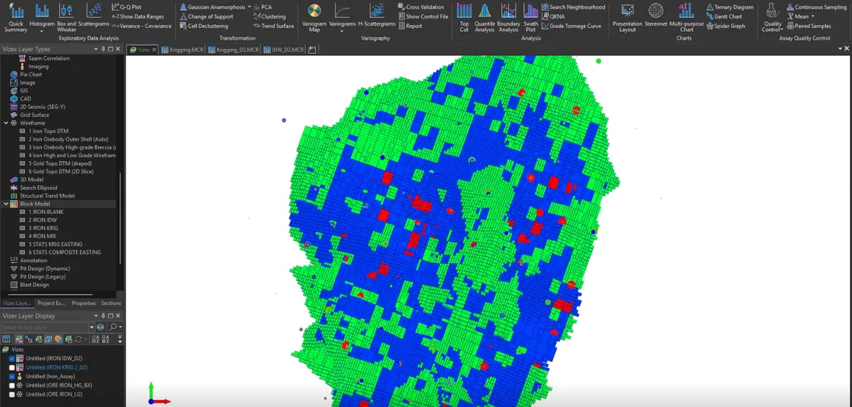
Stage 16 of the Micromine Origin sequence: the principal model components are assembled in a final three-dimensional view for technical review and communication.
ALBUM
55 records
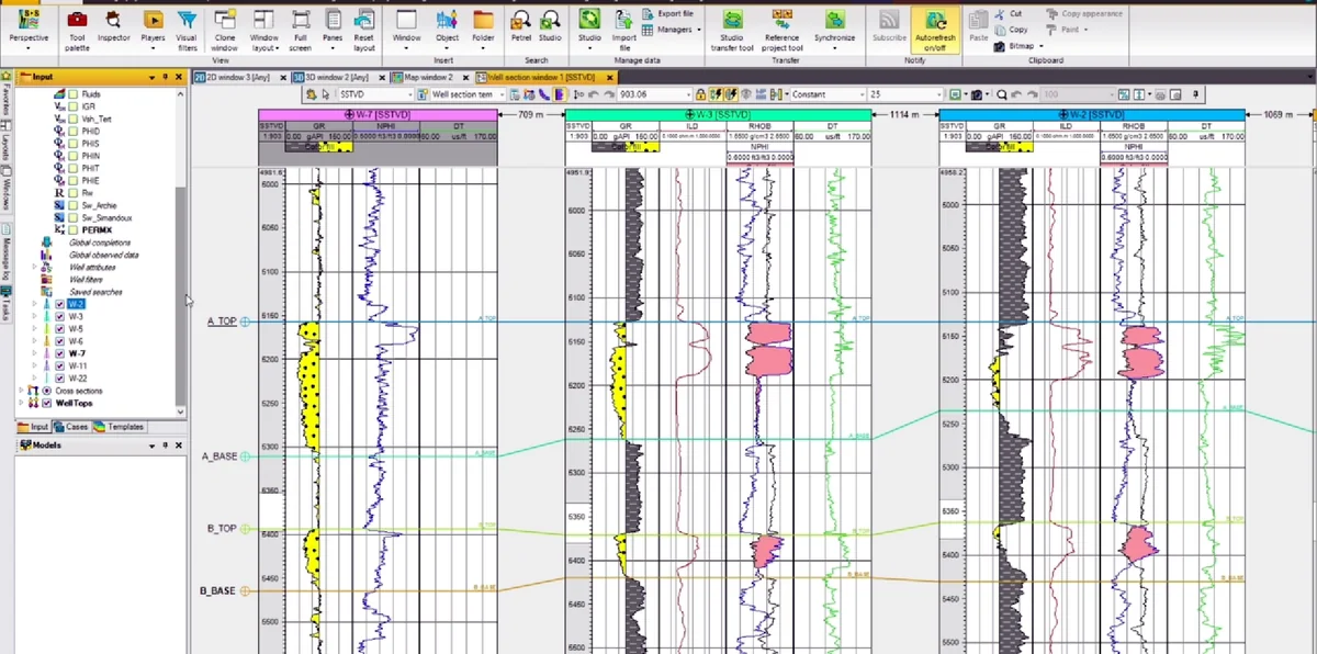
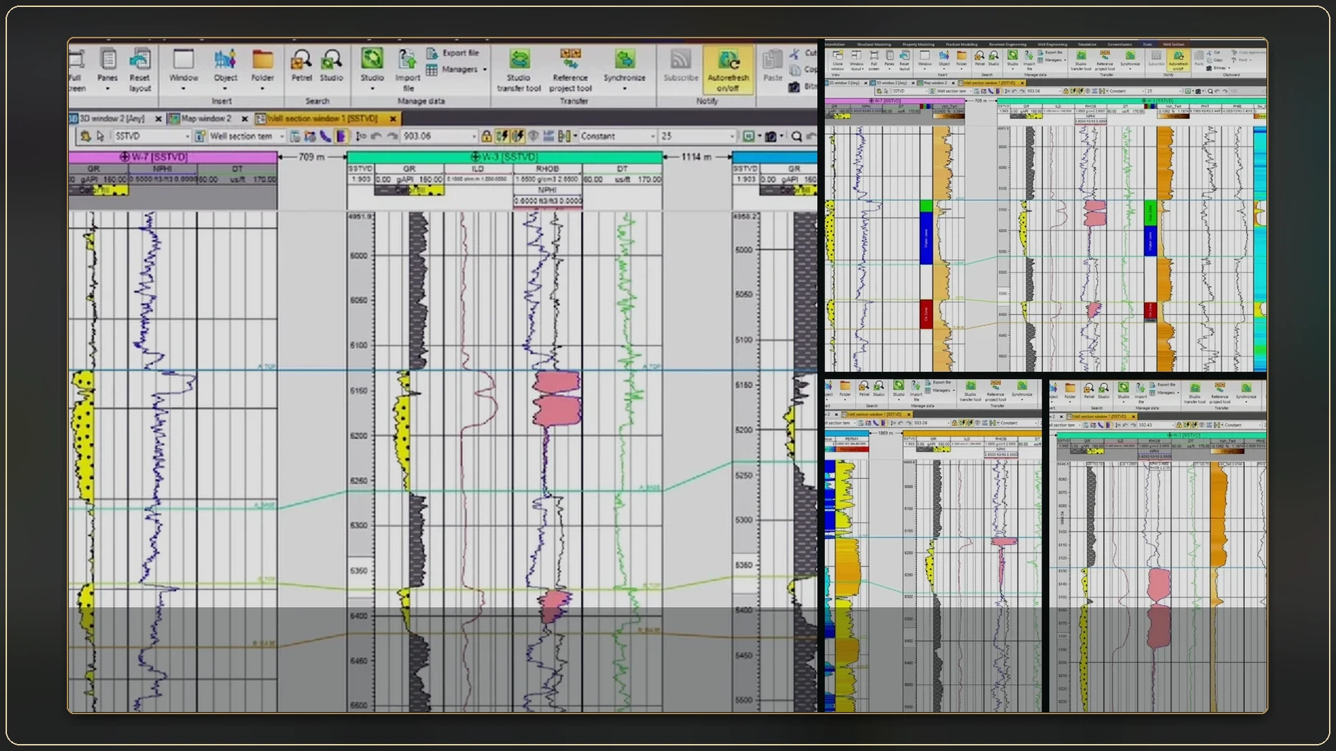
Stage 01 of the Petrel sequence: the Petrel project tree and well-section window are organised so that logs, markers, facies tracks and model objects can be reviewed from a single correlation workspace.
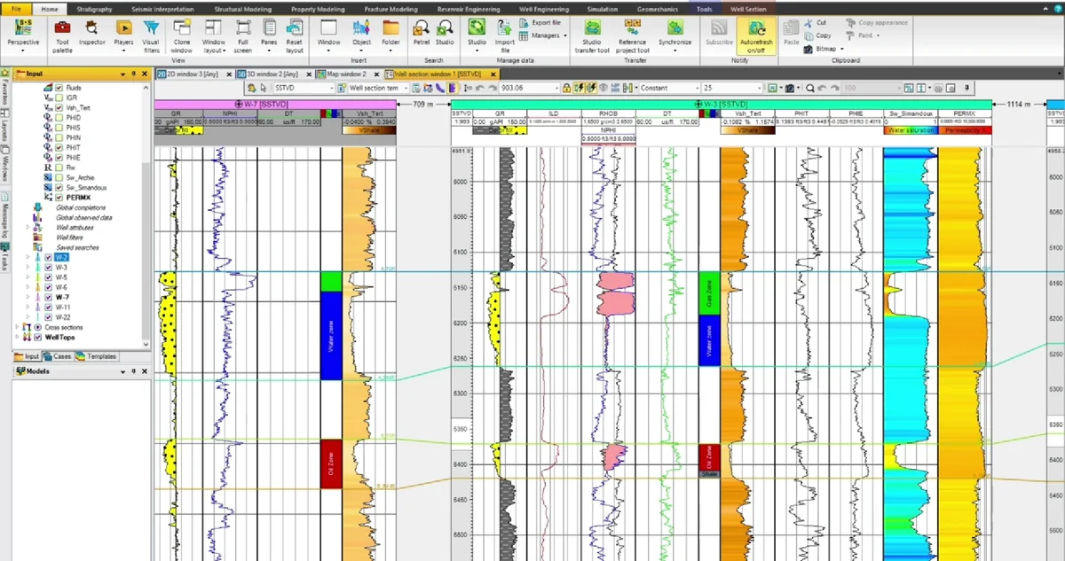
Stage 02 of the Petrel sequence: gamma-ray, density, lithology and interpreted tracks are arranged at a common vertical scale for direct comparison.
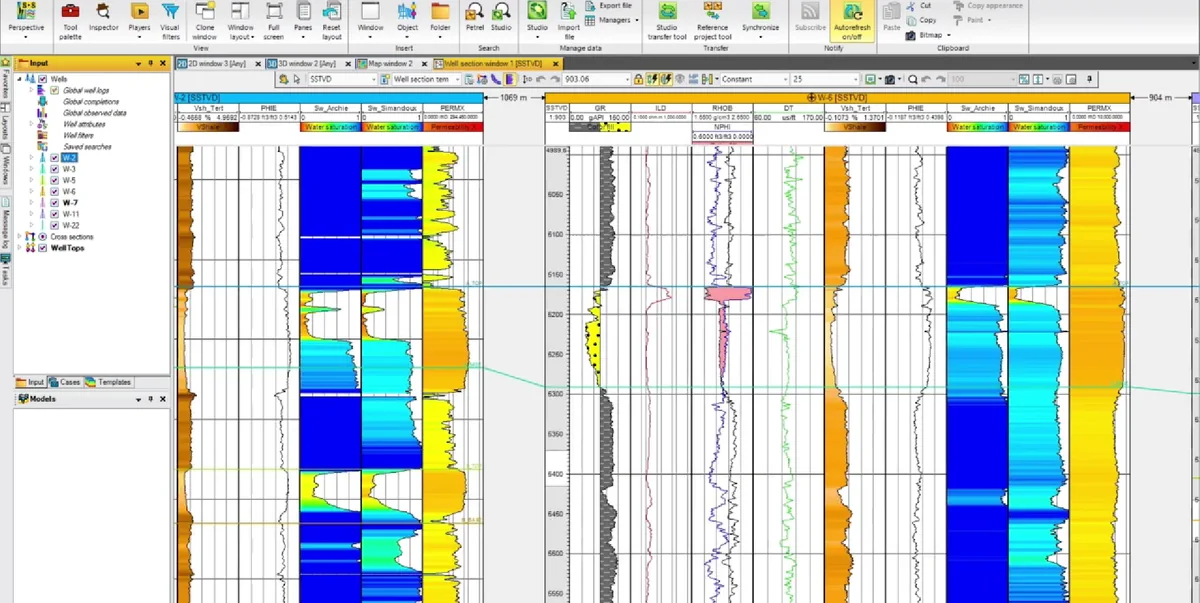
Stage 03 of the Petrel sequence: multiple wells are aligned in one correlation panel, with markers and interpreted intervals connected across the section.
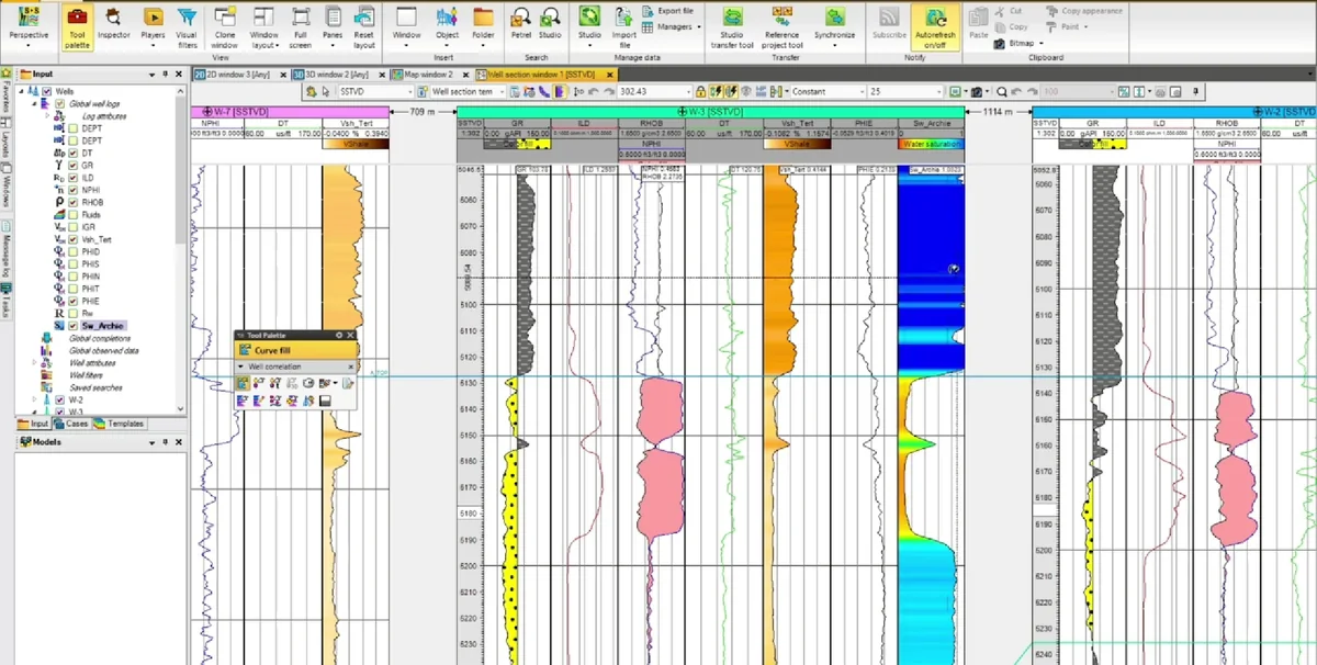
Stage 04 of the Petrel sequence: log curves, marker picks and interval boundaries are adjusted at well scale while neighbouring wells remain visible for control.
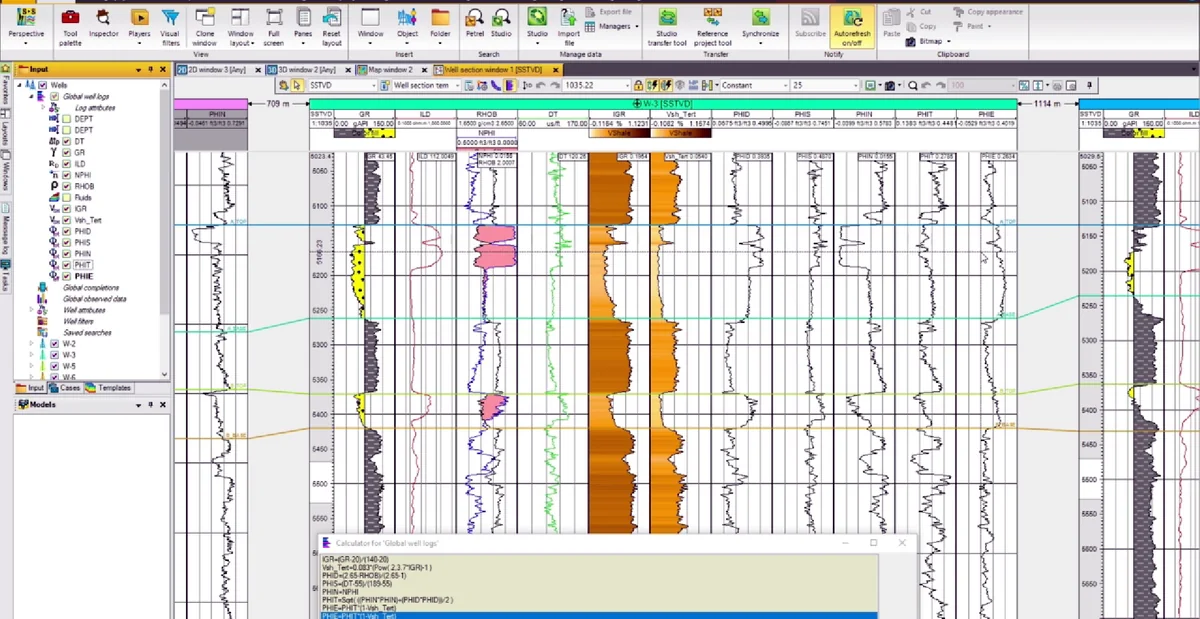
Stage 05 of the Petrel sequence: log curves, marker picks and interval boundaries are adjusted at well scale while neighbouring wells remain visible for control.
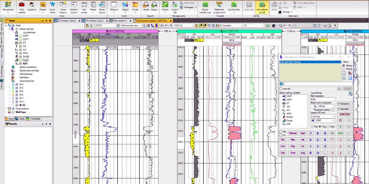
Stage 06 of the Petrel sequence: log curves, marker picks and interval boundaries are adjusted at well scale while neighbouring wells remain visible for control.
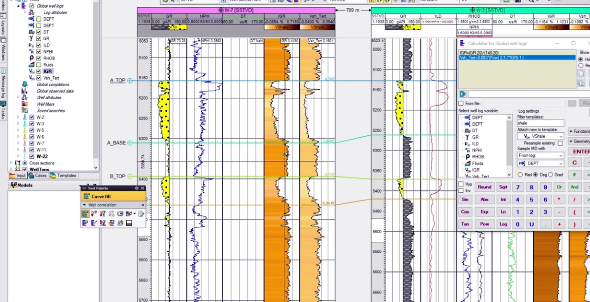
Stage 07 of the Petrel sequence: colour-coded electrofacies or property tracks are inspected beside the wireline logs and correlated markers.
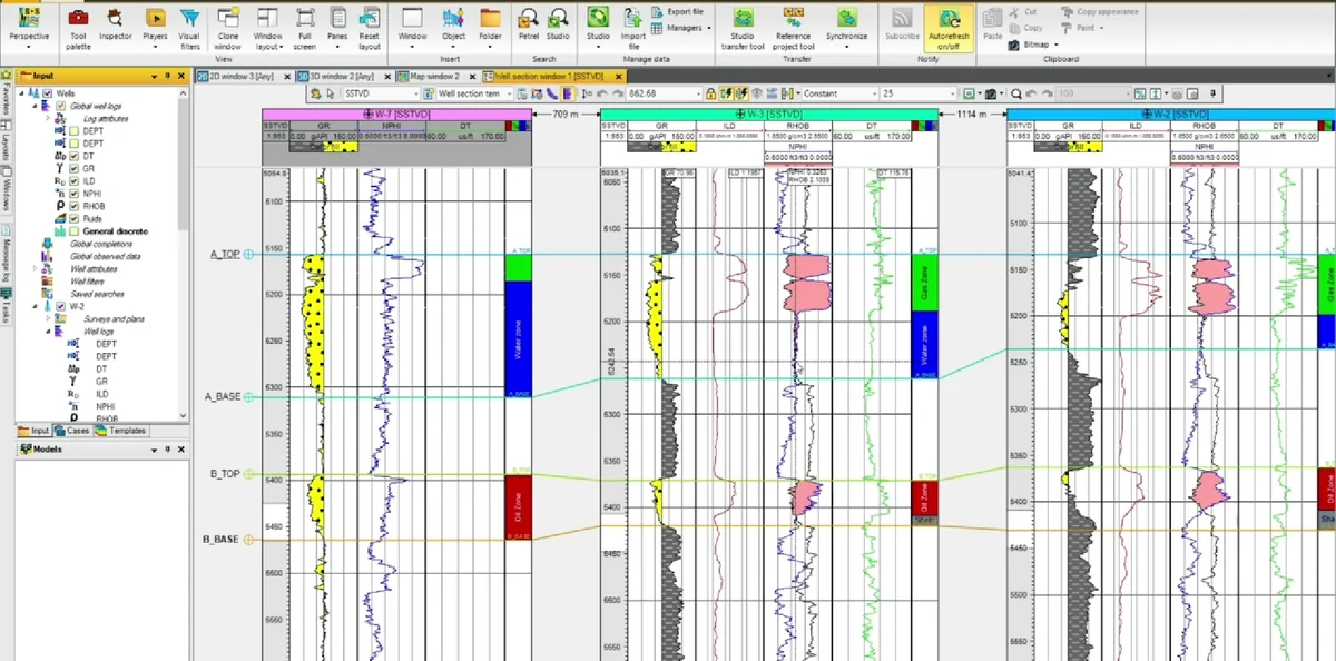
Stage 08 of the Petrel sequence: multiple wells are aligned in one correlation panel, with markers and interpreted intervals connected across the section.
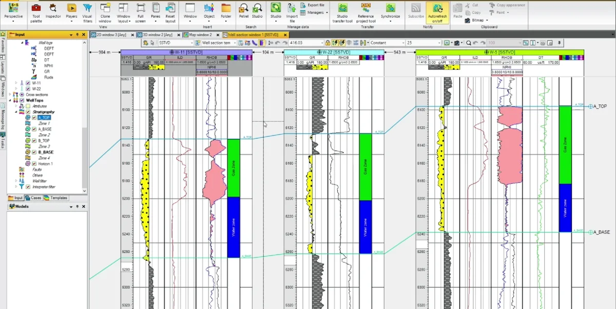
Stage 09 of the Petrel sequence: colour-coded electrofacies or property tracks are inspected beside the wireline logs and correlated markers.
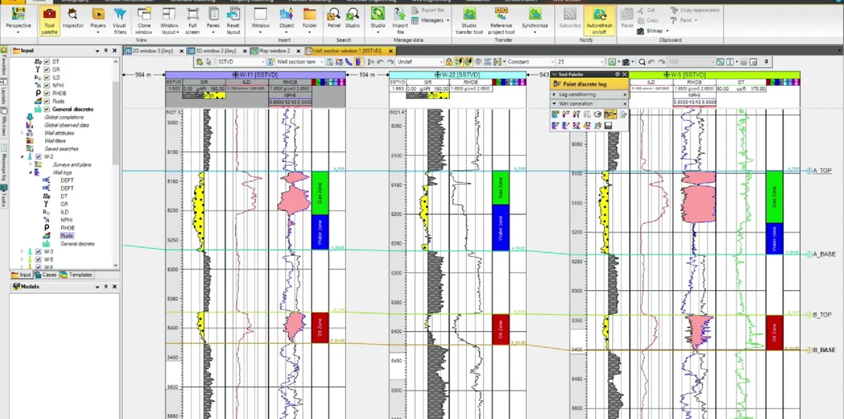
Stage 10 of the Petrel sequence: multiple wells are aligned in one correlation panel, with markers and interpreted intervals connected across the section.
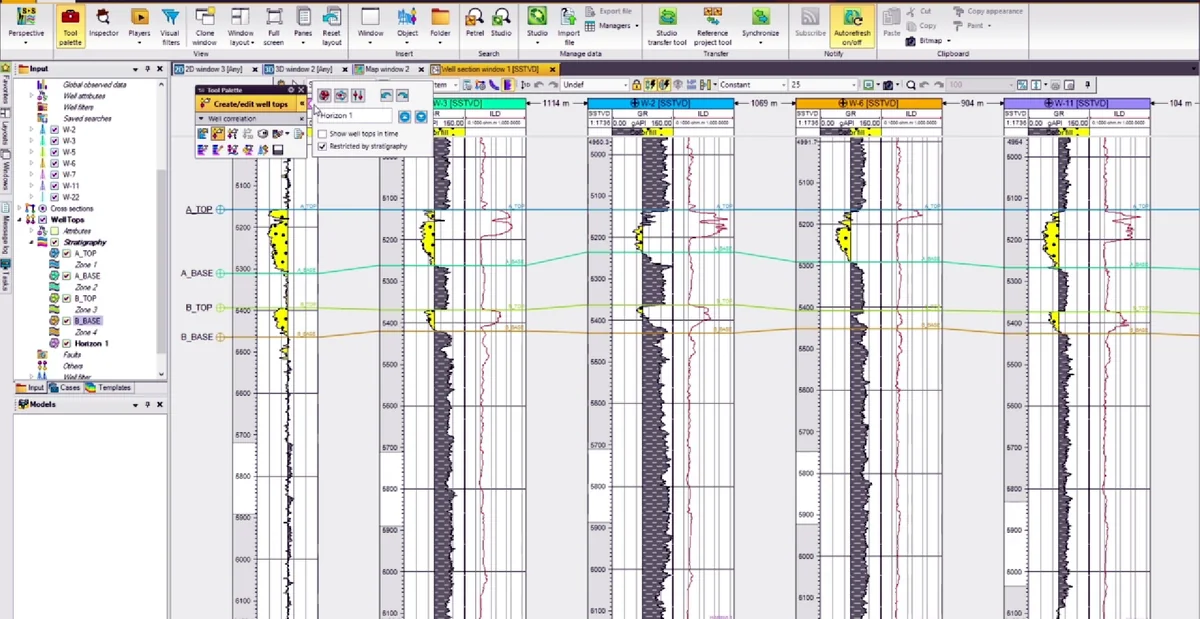
Stage 11 of the Petrel sequence: the correlated wells are positioned within a three-dimensional structural context to check the spatial relationship between the section and the model framework.
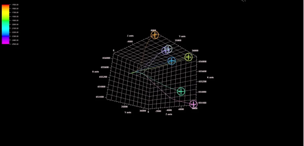
Stage 12 of the Petrel sequence: a three-dimensional surface or horizon object is isolated to inspect its geometry relative to the available well control.
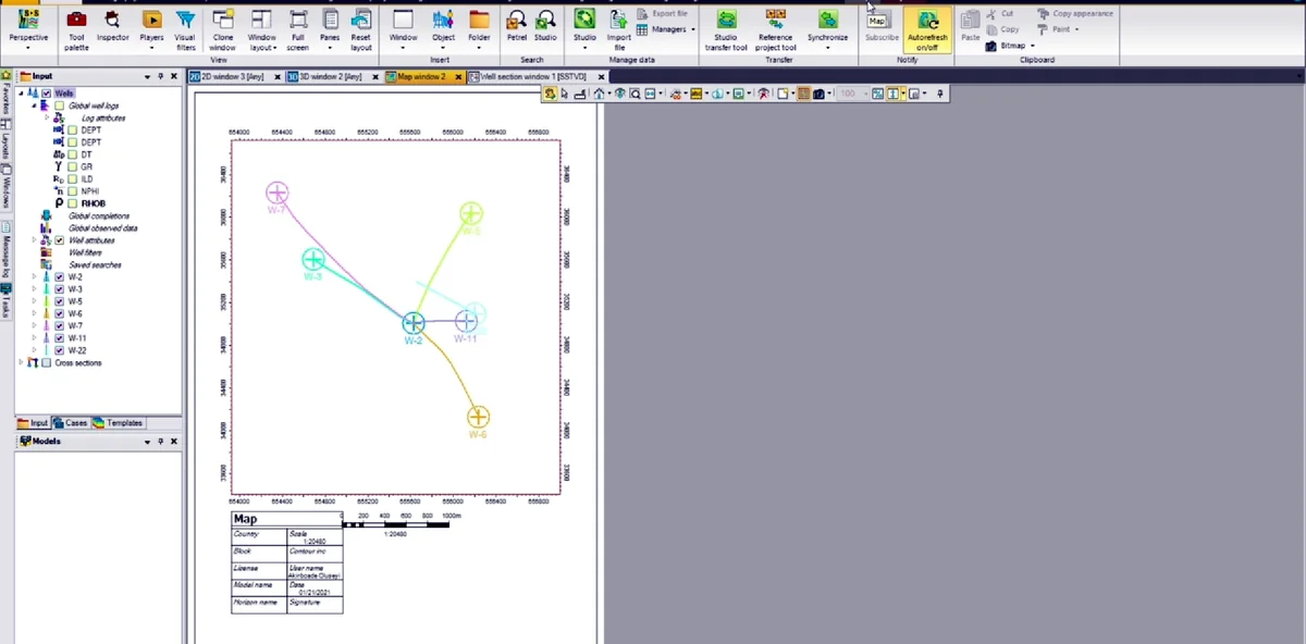
Stage 13 of the Petrel sequence: a diagnostic plot and project controls are used to review the consistency of the interpreted model against the available data.
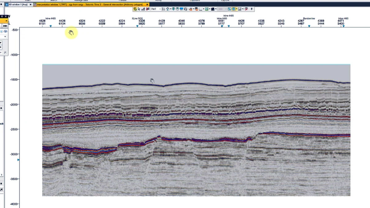
Stage 14 of the Petrel sequence: a vertical seismic section carries several interpreted horizons, allowing reflector continuity and structural relief to be followed along one line.
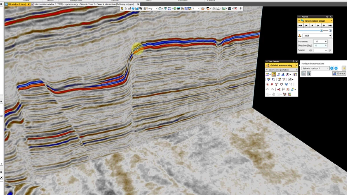
Stage 15 of the Petrel sequence: intersecting seismic panels display the same interpreted horizons from different directions, exposing misties and inconsistent picks at line intersections.
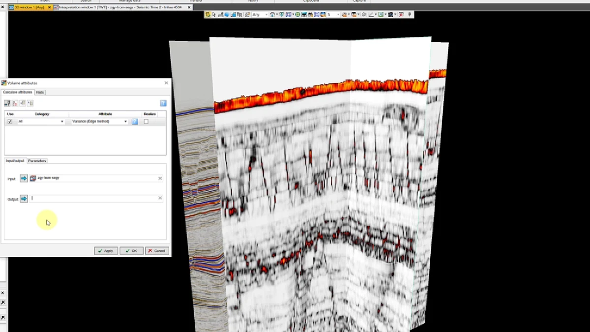
Stage 16 of the Petrel sequence: intersecting seismic panels display the same interpreted horizons from different directions, exposing misties and inconsistent picks at line intersections.
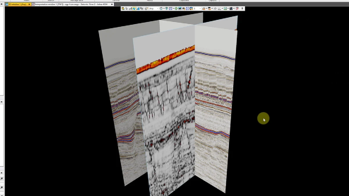
Stage 17 of the Petrel sequence: intersecting seismic panels display the same interpreted horizons from different directions, exposing misties and inconsistent picks at line intersections.
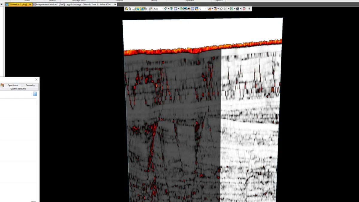
Stage 18 of the Petrel sequence: display opacity and colour controls are adjusted while the seismic volume and interpretation remain visible.
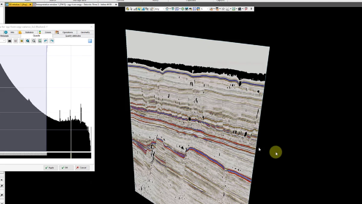
Stage 19 of the Petrel sequence: interpreted horizons are traced across a vertical seismic section, including intervals where reflector continuity is disrupted.
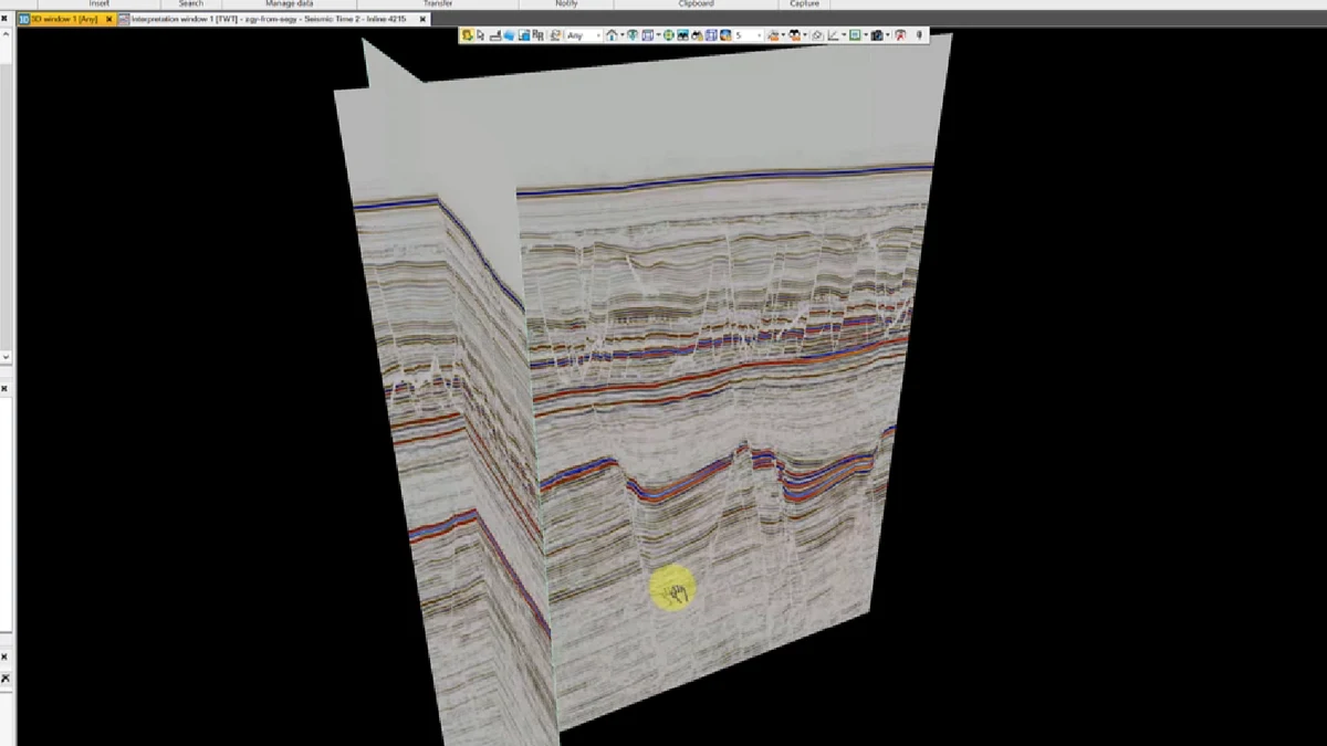
Stage 20 of the Petrel sequence: intersecting seismic panels display the same interpreted horizons from different directions, exposing misties and inconsistent picks at line intersections.
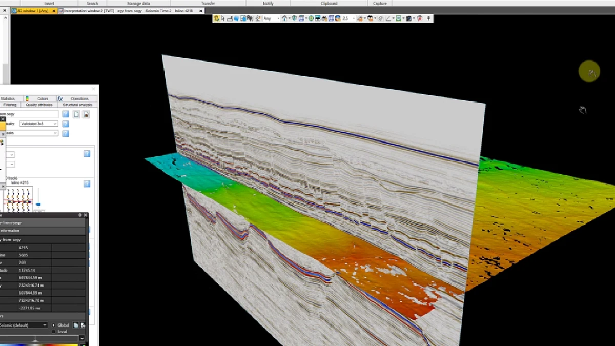
Stage 21 of the Petrel sequence: the interpreted horizon is converted to a colour-ramped surface and viewed together with the seismic control from which it was derived.
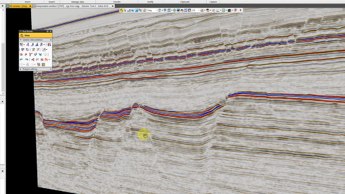
Stage 22 of the Petrel sequence: interpreted horizons are traced across a vertical seismic section, including intervals where reflector continuity is disrupted.
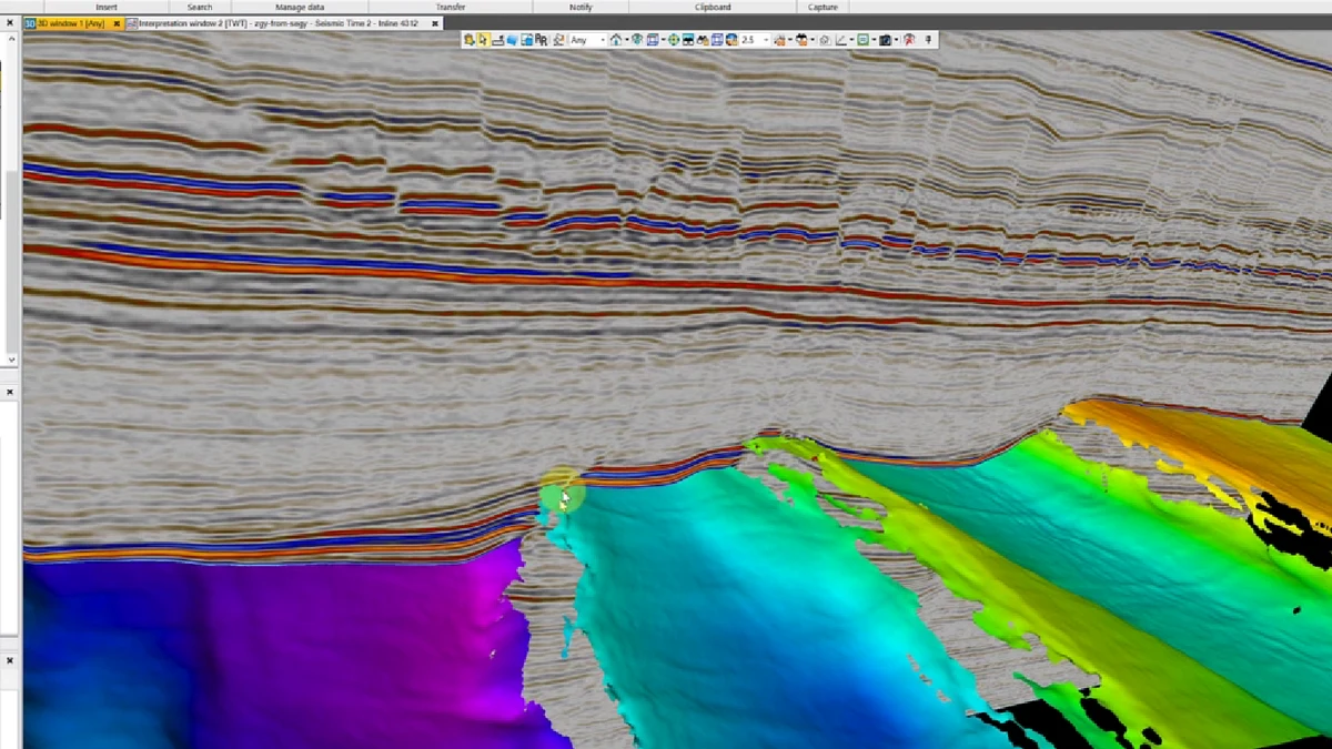
Stage 23 of the Petrel sequence: the interpreted horizon is converted to a colour-ramped surface and viewed together with the seismic control from which it was derived.
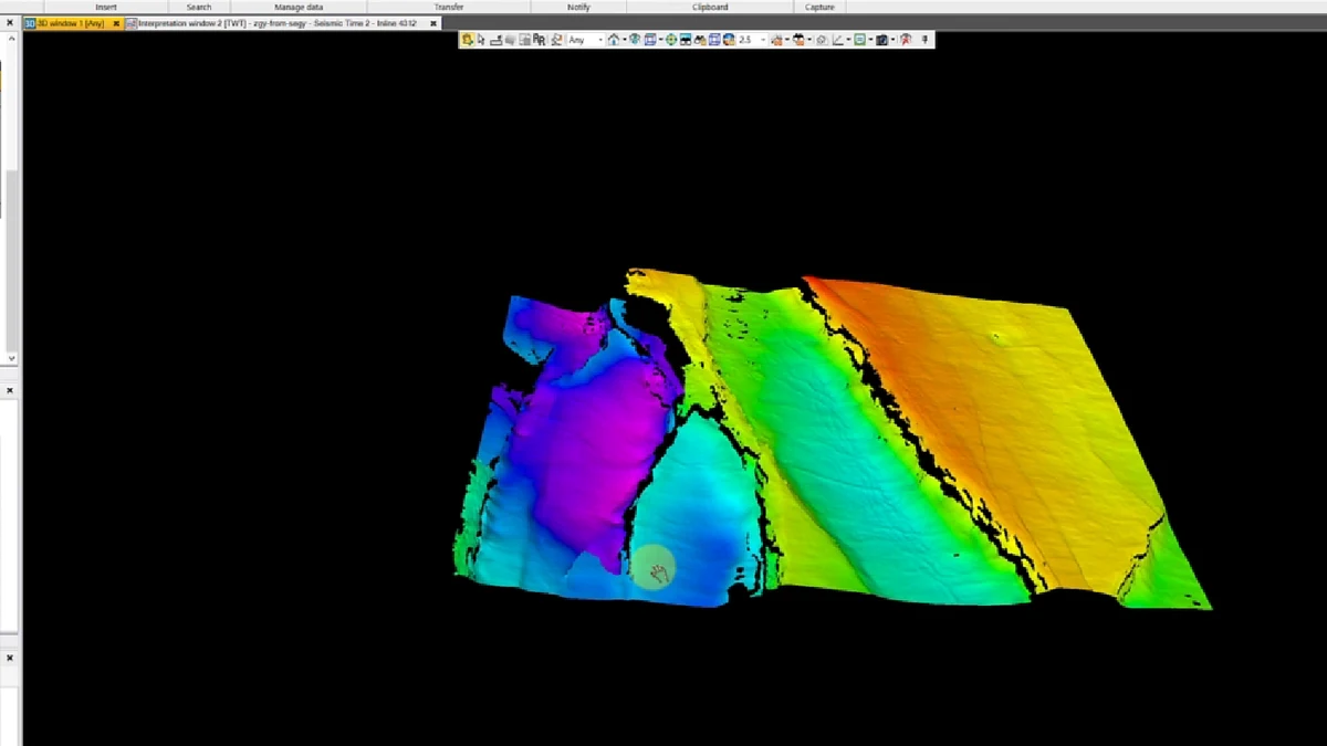
Stage 24 of the Petrel sequence: the interpreted horizon is converted to a colour-ramped surface and viewed together with the seismic control from which it was derived.
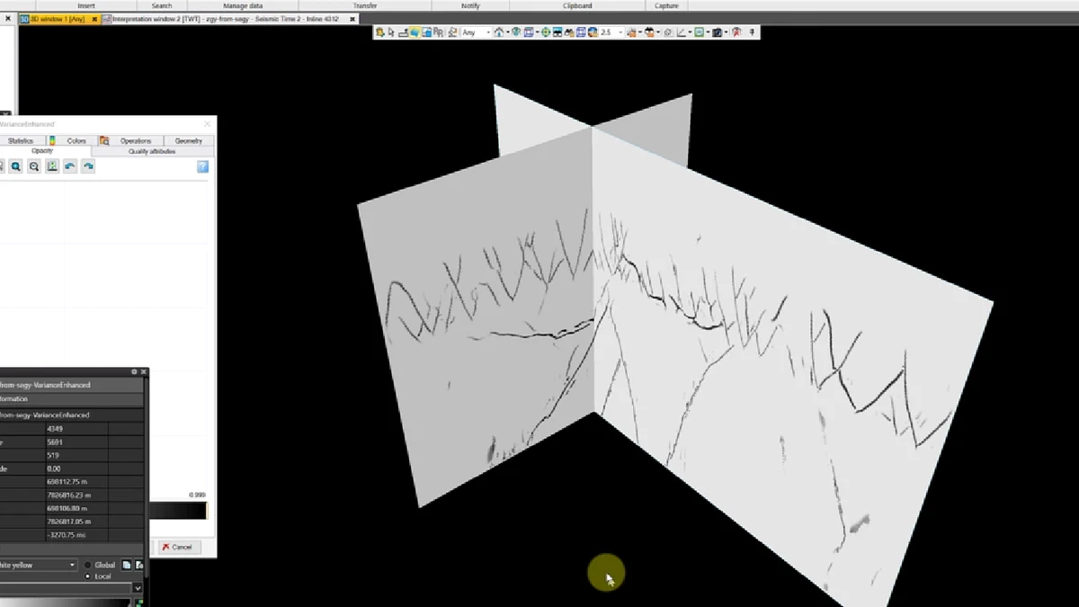
Stage 25 of the Petrel sequence: fault traces and fault sticks are displayed on orthogonal seismic panels, with horizon offsets providing structural control.
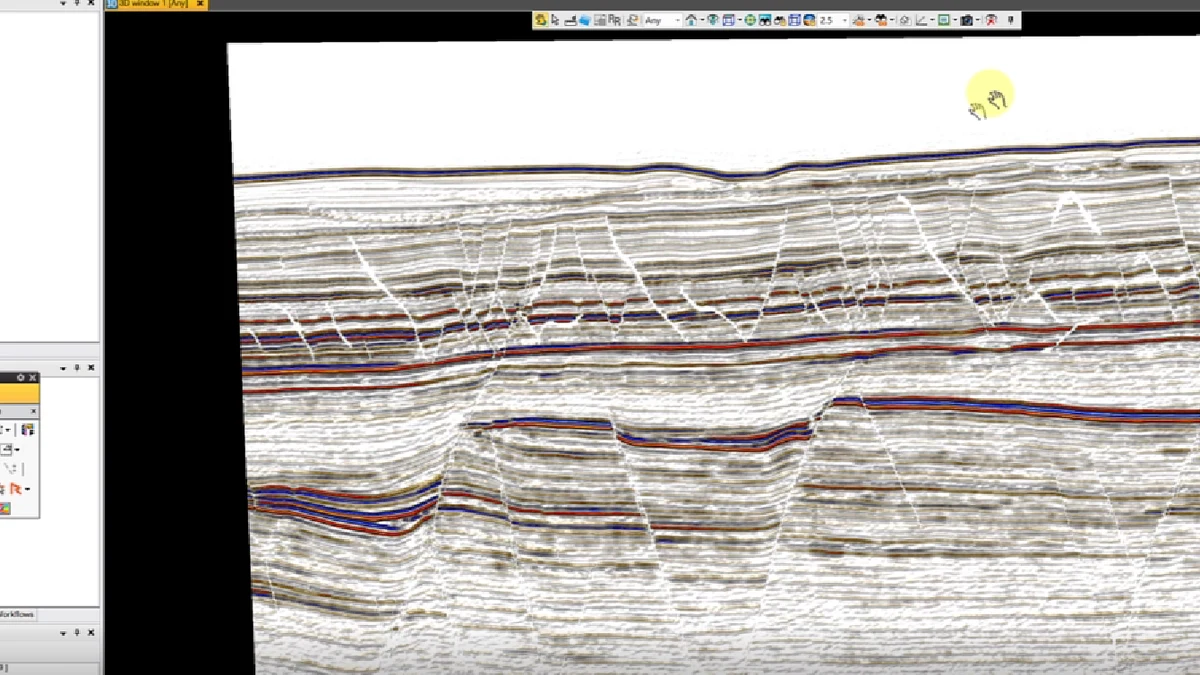
Stage 26 of the Petrel sequence: fault traces and fault sticks are displayed on orthogonal seismic panels, with horizon offsets providing structural control.
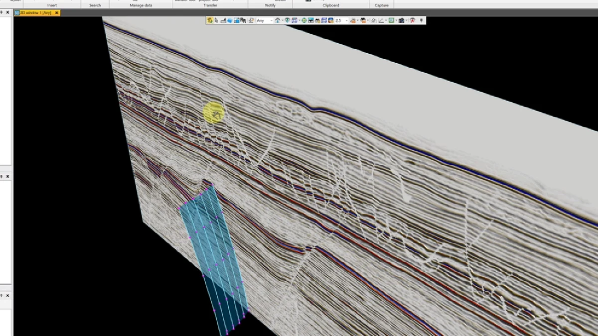
Stage 27 of the Petrel sequence: a single fault surface is positioned against the seismic and horizon framework to review its dip, extent and intersection geometry.
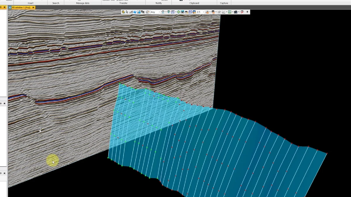
Stage 28 of the Petrel sequence: a single fault surface is positioned against the seismic and horizon framework to review its dip, extent and intersection geometry.
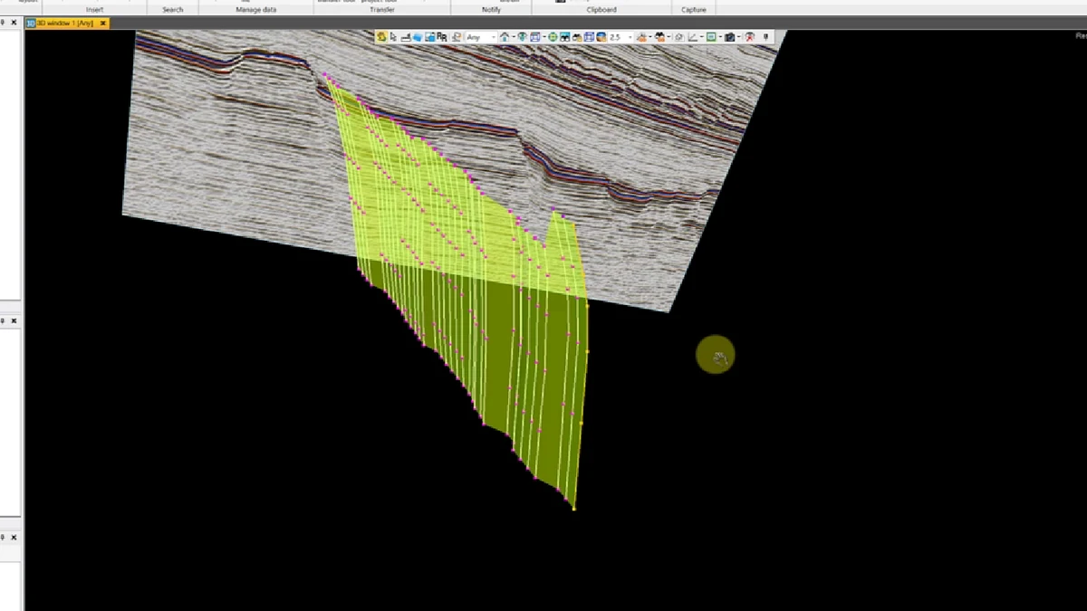
Stage 29 of the Petrel sequence: a single fault surface is positioned against the seismic and horizon framework to review its dip, extent and intersection geometry.
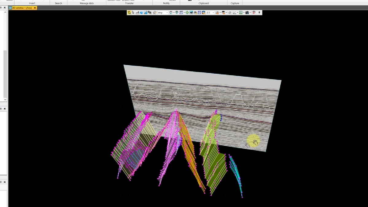
Stage 30 of the Petrel sequence: multiple fault-stick sets are assembled in three dimensions, revealing segmentation, overlap and the structural density of the interpreted network.
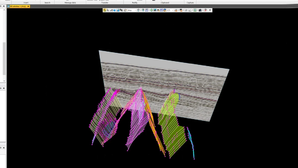
Stage 31 of the Petrel sequence: multiple fault-stick sets are assembled in three dimensions, revealing segmentation, overlap and the structural density of the interpreted network.
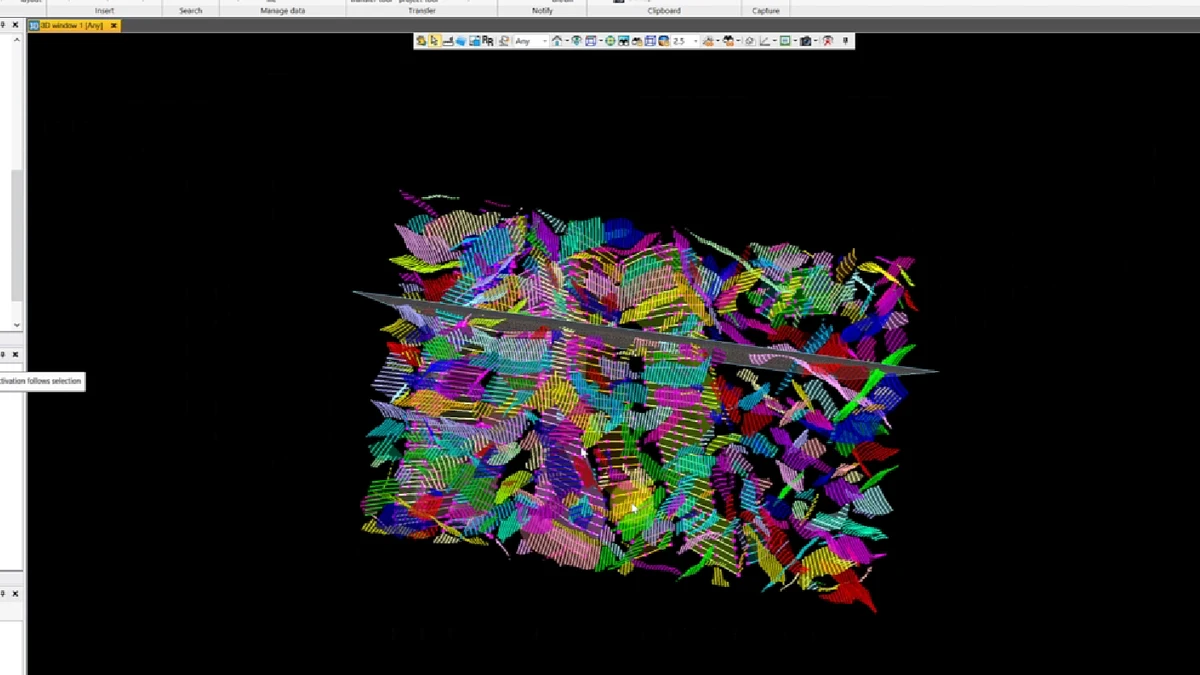
Stage 32 of the Petrel sequence: multiple fault-stick sets are assembled in three dimensions, revealing segmentation, overlap and the structural density of the interpreted network.
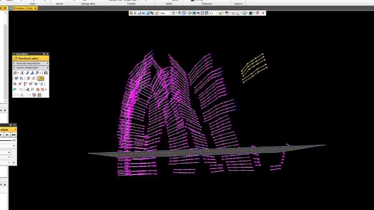
Stage 33 of the Petrel sequence: multiple fault-stick sets are assembled in three dimensions, revealing segmentation, overlap and the structural density of the interpreted network.
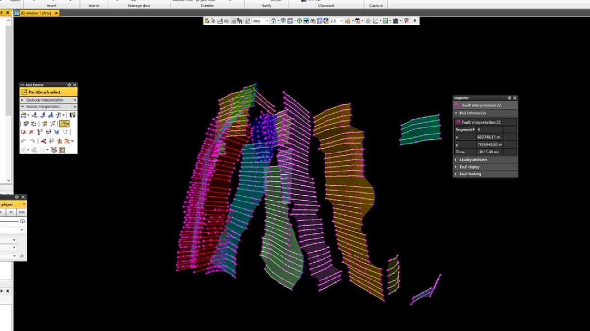
Stage 34 of the Petrel sequence: colour-coded fault surfaces have been generated from the interpreted stick sets, allowing individual structures and intersections to be distinguished.
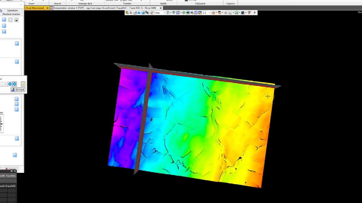
Stage 35 of the Petrel sequence: a colour-ramped structural surface is inspected in map view to identify relief, lineaments and fault-controlled discontinuities.
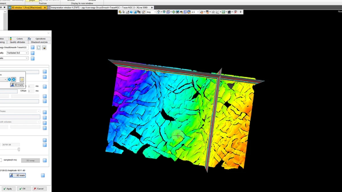
Stage 36 of the Petrel sequence: a colour-ramped structural surface is inspected in map view to identify relief, lineaments and fault-controlled discontinuities.
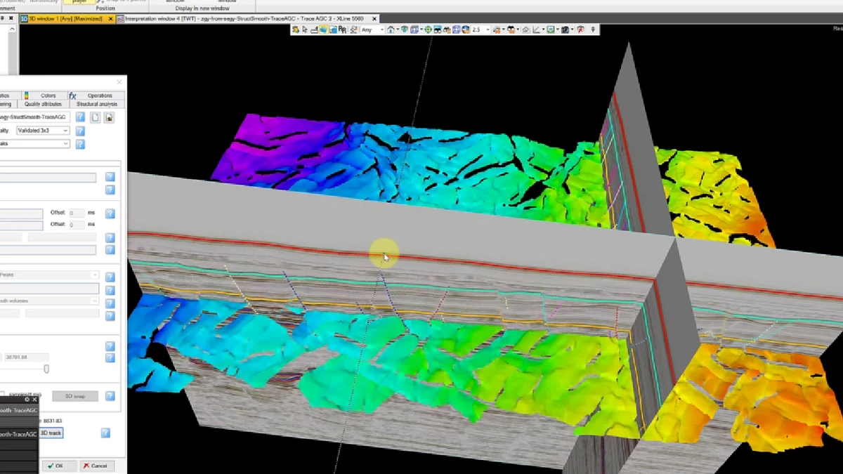
Stage 37 of the Petrel sequence: the mapped surface is intersected by vertical seismic panels, tying surface morphology back to the interpreted reflectors and faults.
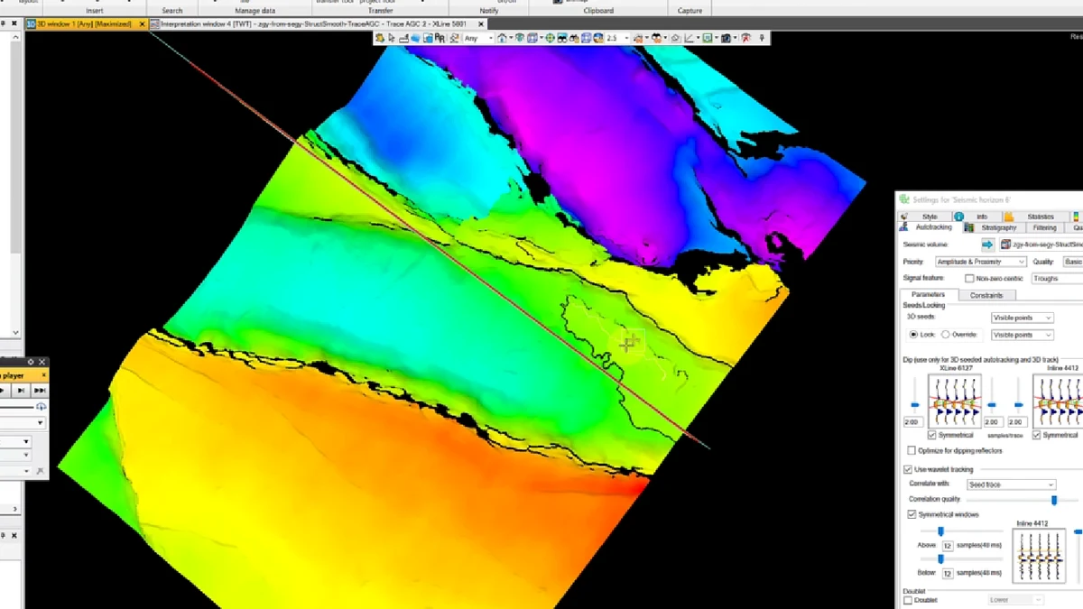
Stage 38 of the Petrel sequence: a colour-ramped structural surface is inspected in map view to identify relief, lineaments and fault-controlled discontinuities.
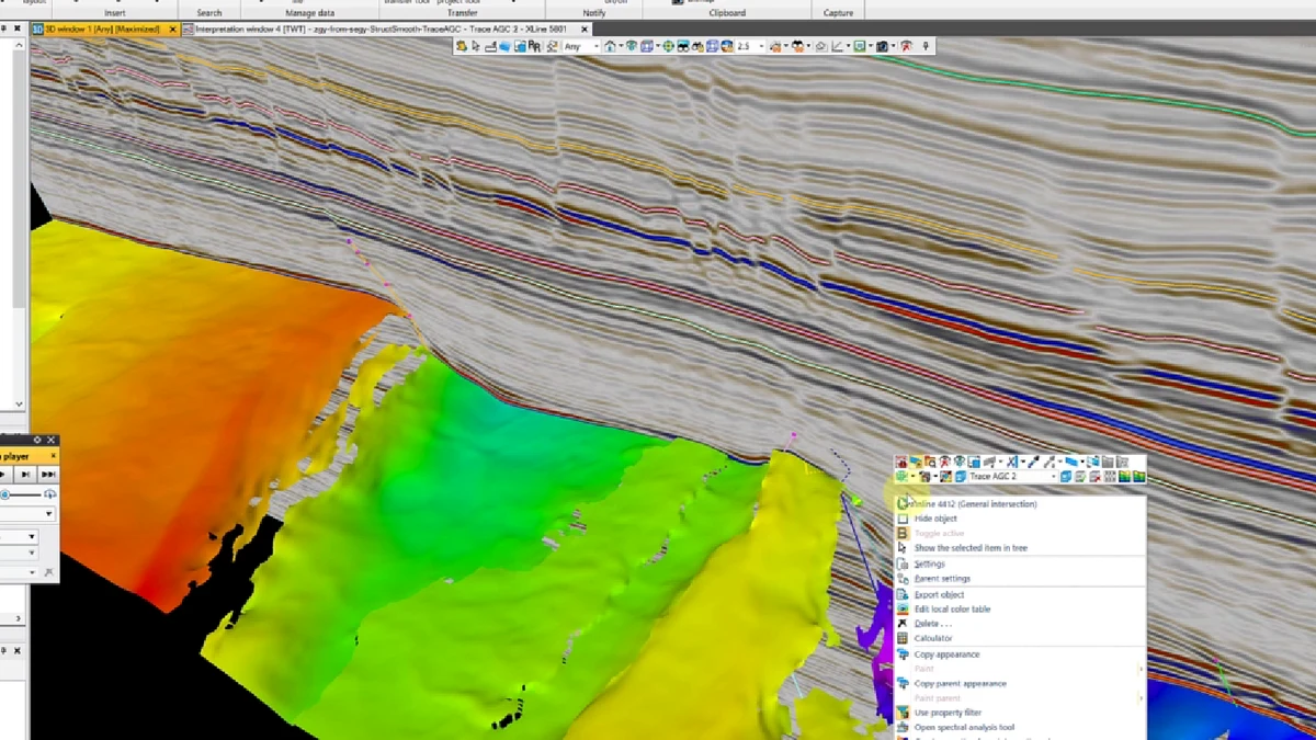
Stage 39 of the Petrel sequence: the mapped surface is intersected by vertical seismic panels, tying surface morphology back to the interpreted reflectors and faults.
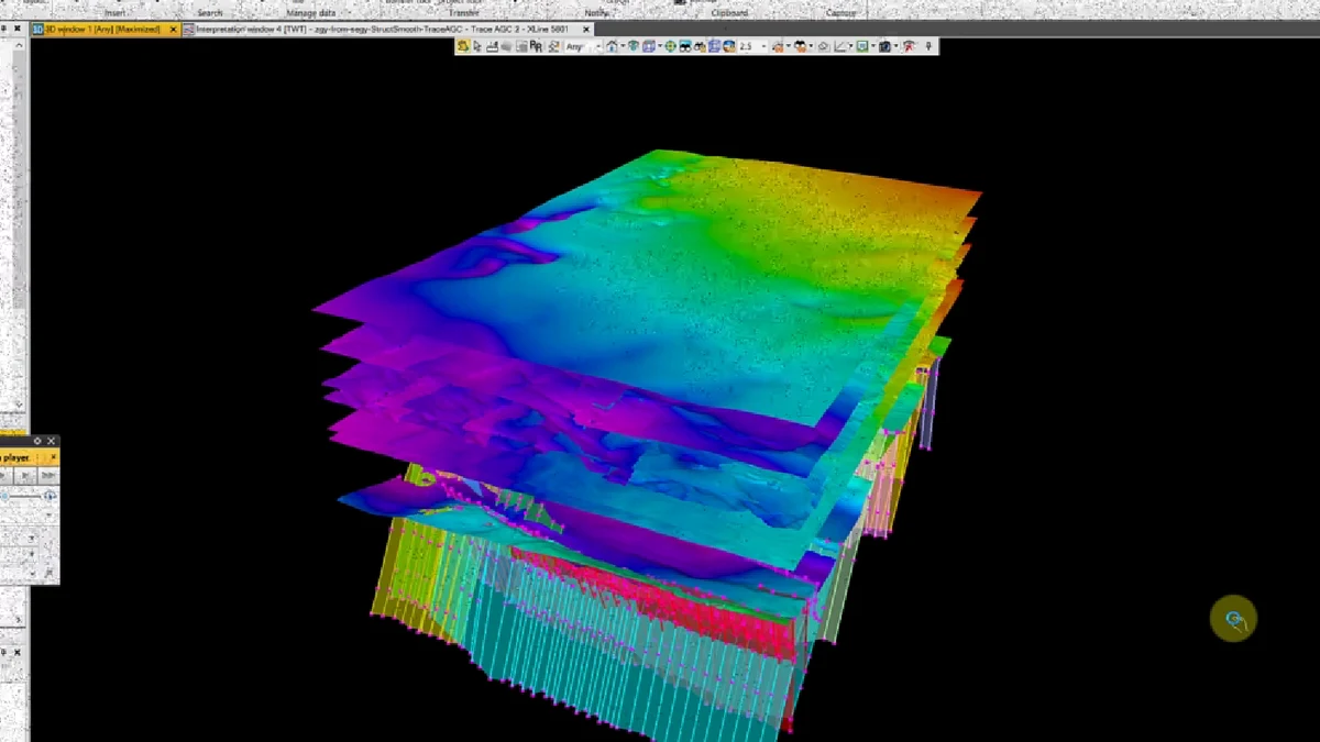
Stage 40 of the Petrel sequence: seismic panels, interpreted horizons and fault surfaces are displayed together in the final three-dimensional structural scene.
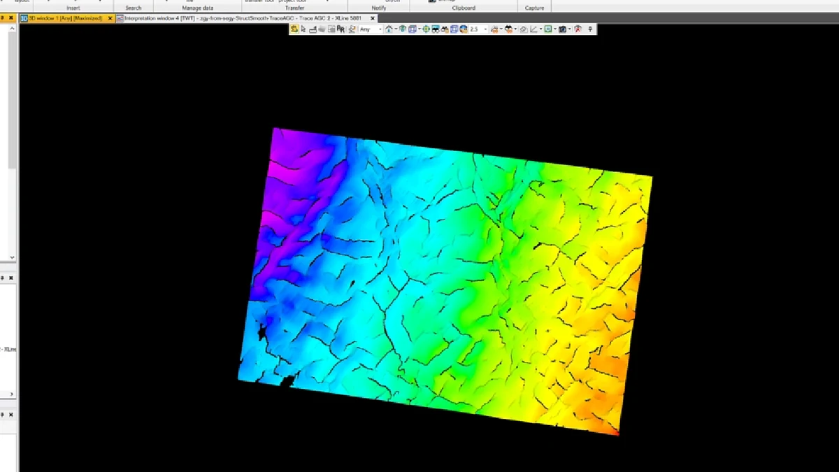
Stage 41 of the Petrel sequence: a colour-ramped structural surface is inspected in map view to identify relief, lineaments and fault-controlled discontinuities.
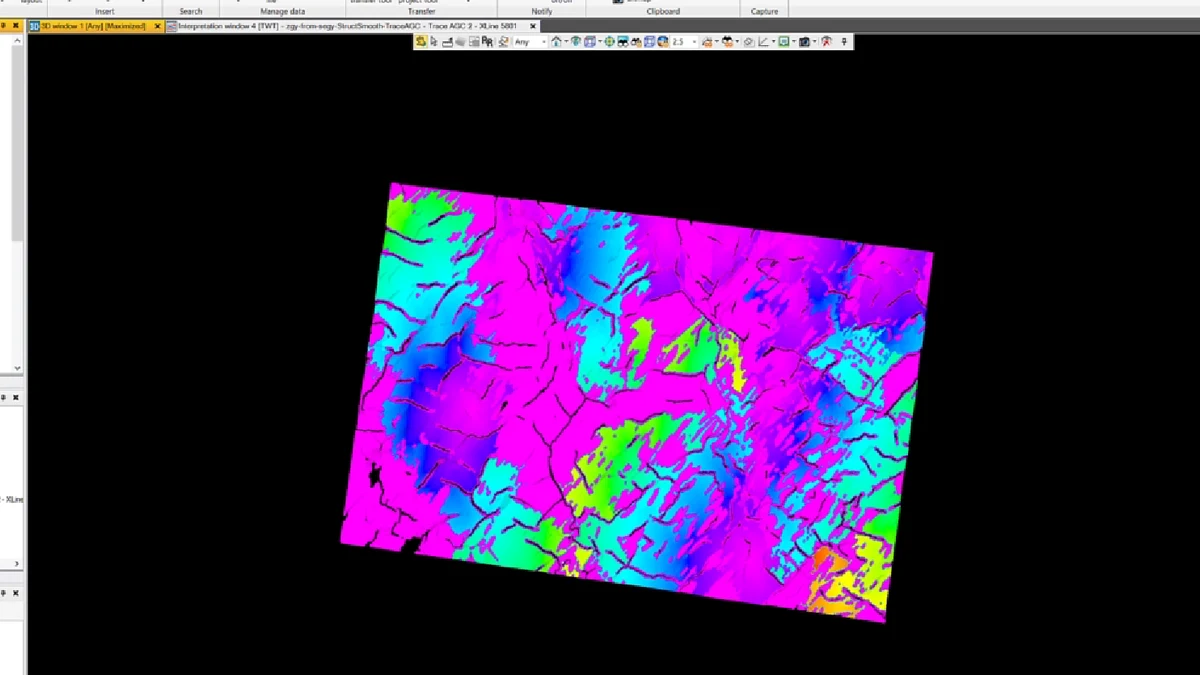
Stage 42 of the Petrel sequence: a derived surface attribute is displayed continuously and categorically to emphasise lineaments, local relief changes and structural texture.
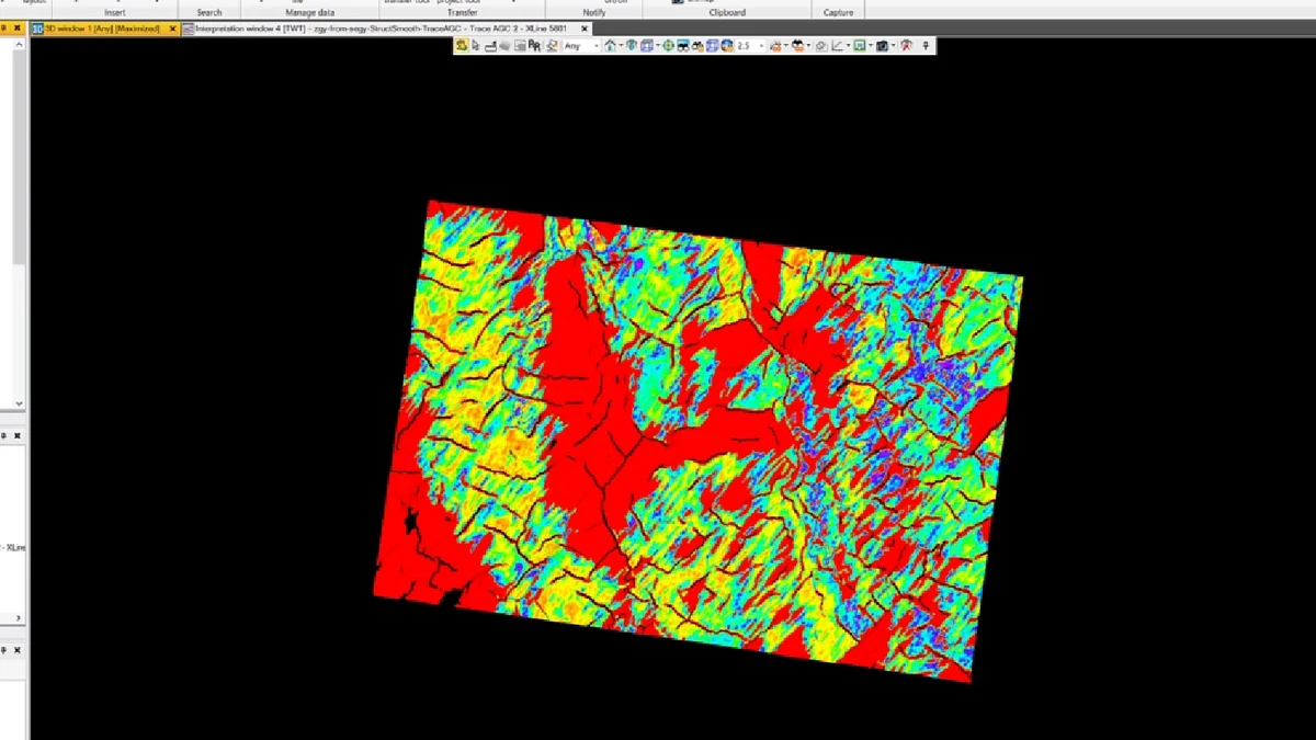
Stage 43 of the Petrel sequence: a derived surface attribute is displayed continuously and categorically to emphasise lineaments, local relief changes and structural texture.
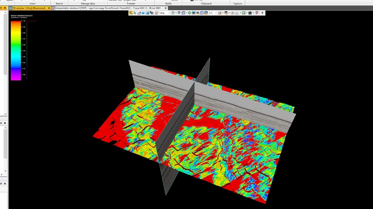
Stage 44 of the Petrel sequence: the mapped surface is intersected by vertical seismic panels, tying surface morphology back to the interpreted reflectors and faults.
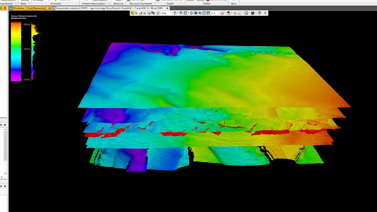
Stage 45 of the Petrel sequence: several interpreted horizon surfaces are stacked and contoured to review stratigraphic order, vertical separation and local surface shape.
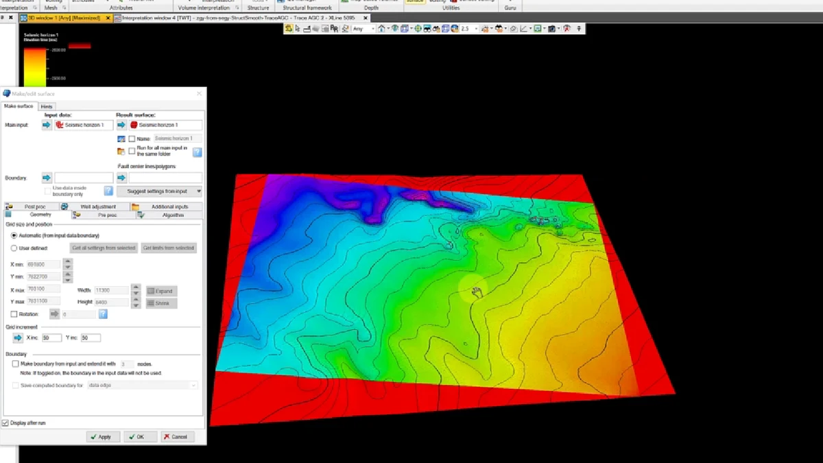
Stage 46 of the Petrel sequence: several interpreted horizon surfaces are stacked and contoured to review stratigraphic order, vertical separation and local surface shape.
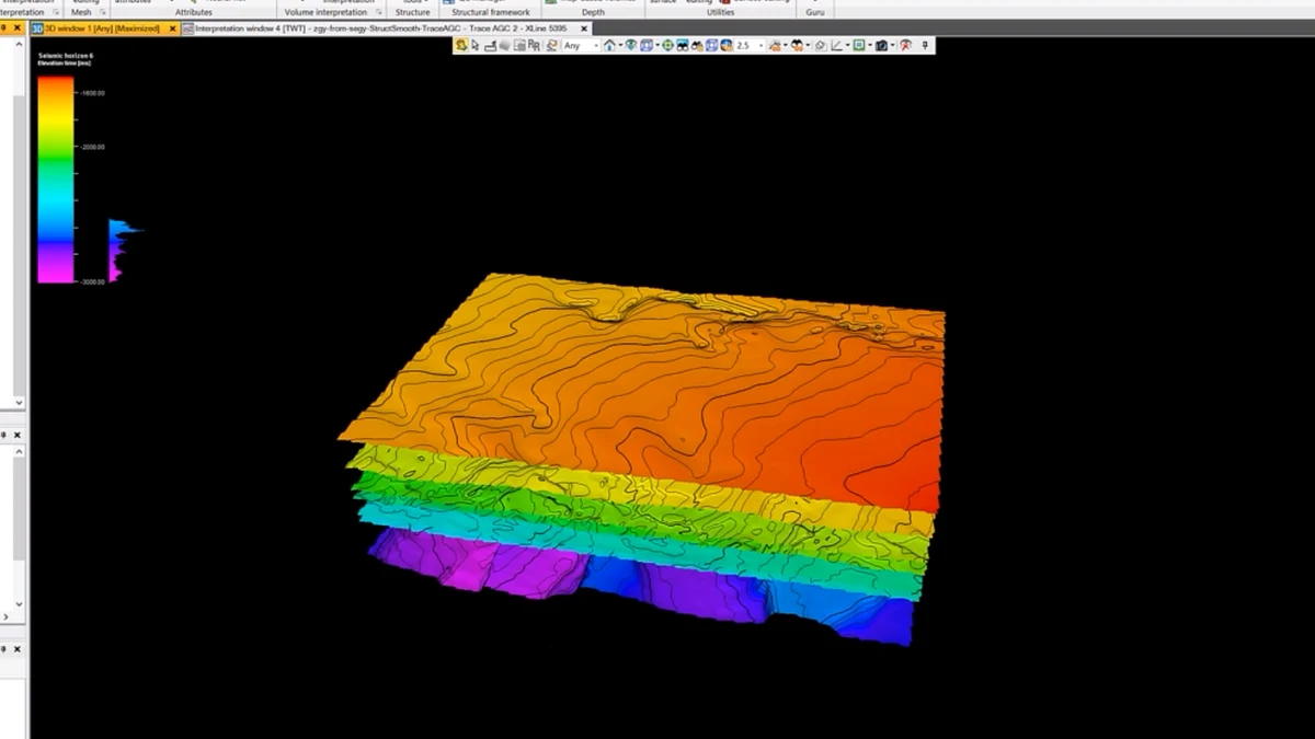
Stage 47 of the Petrel sequence: several interpreted horizon surfaces are stacked and contoured to review stratigraphic order, vertical separation and local surface shape.
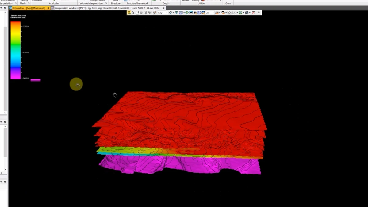
Stage 48 of the Petrel sequence: several interpreted horizon surfaces are stacked and contoured to review stratigraphic order, vertical separation and local surface shape.
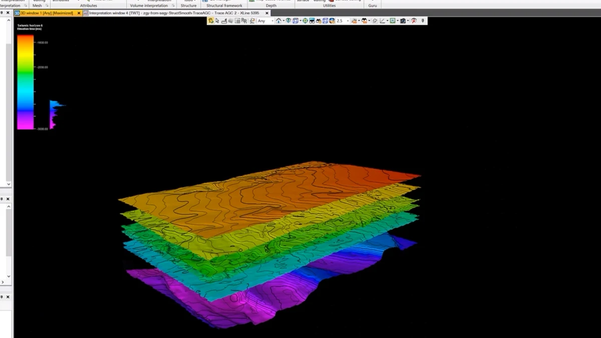
Stage 49 of the Petrel sequence: several interpreted horizon surfaces are stacked and contoured to review stratigraphic order, vertical separation and local surface shape.
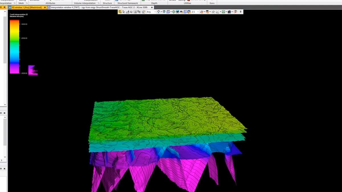
Stage 50 of the Petrel sequence: the fault framework is combined with overlying horizons or a grid-based structural surface, forming the principal geometry of the model.
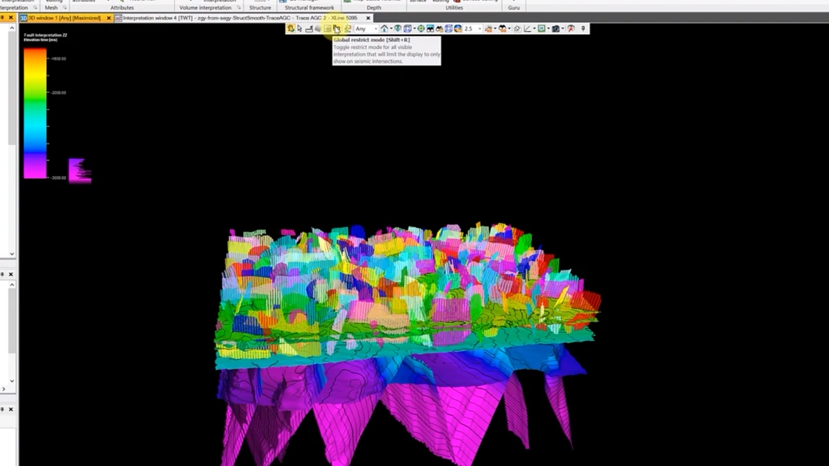
Stage 51 of the Petrel sequence: the fault framework is combined with overlying horizons or a grid-based structural surface, forming the principal geometry of the model.
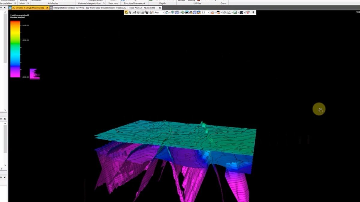
Stage 52 of the Petrel sequence: the fault framework is combined with overlying horizons or a grid-based structural surface, forming the principal geometry of the model.
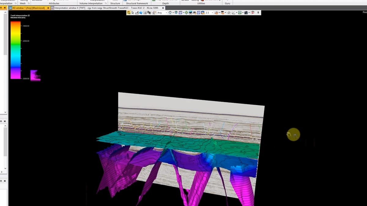
Stage 53 of the Petrel sequence: seismic panels, interpreted horizons and fault surfaces are displayed together in the final three-dimensional structural scene.
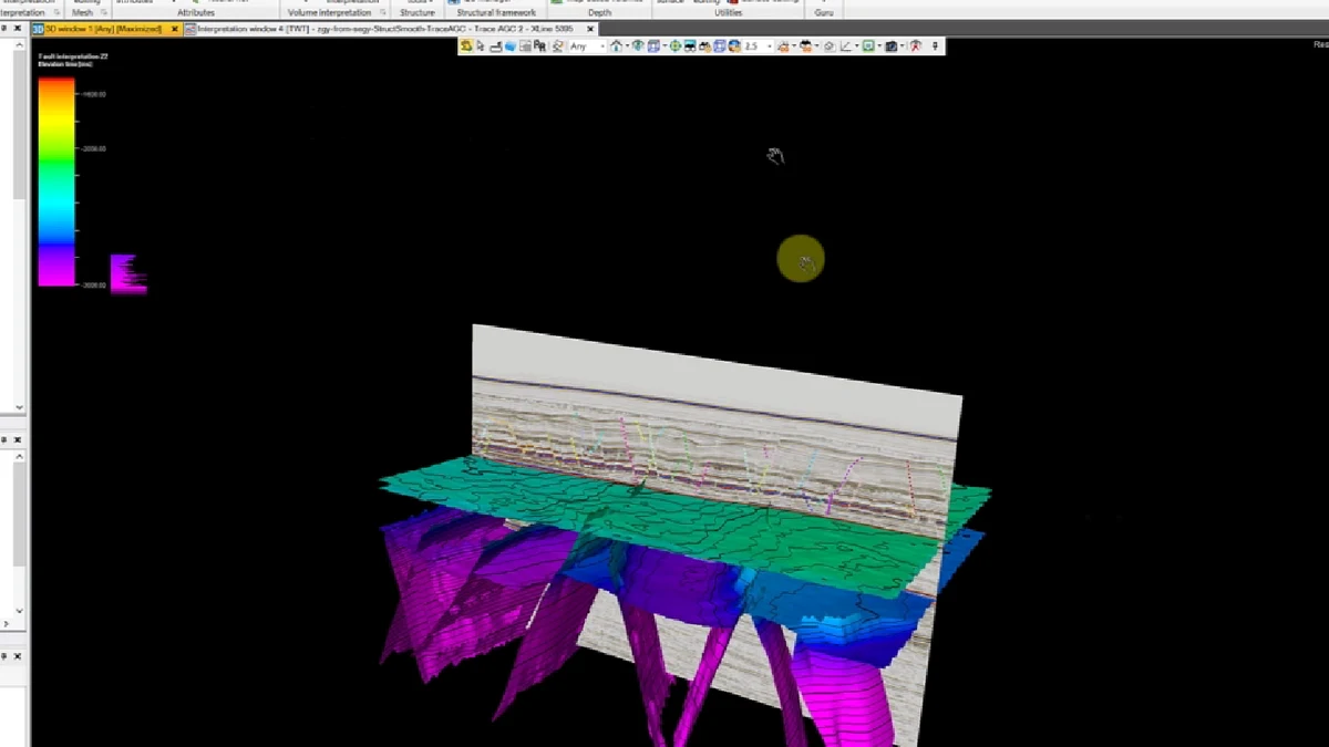
Stage 54 of the Petrel sequence: seismic panels, interpreted horizons and fault surfaces are displayed together in the final three-dimensional structural scene.
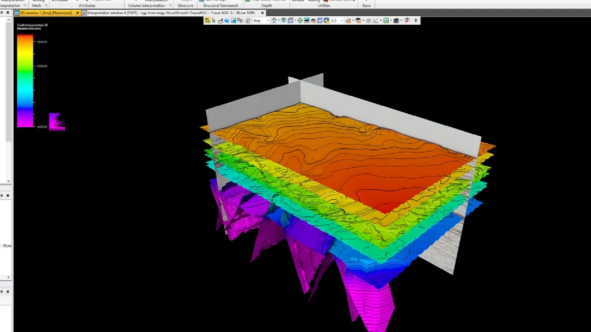
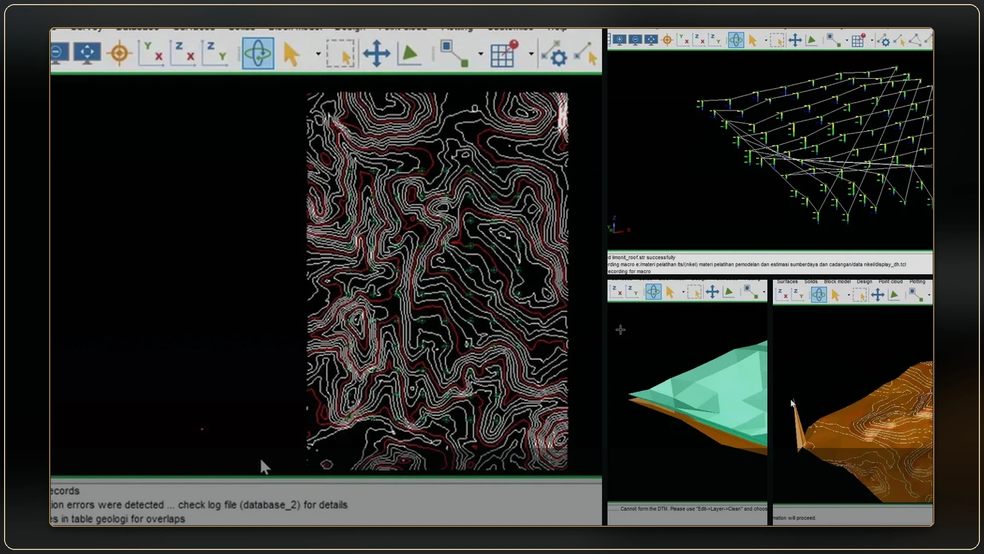
Stage 55 of the Petrel sequence: seismic panels, interpreted horizons and fault surfaces are displayed together in the final three-dimensional structural scene.
ALBUM
17 records
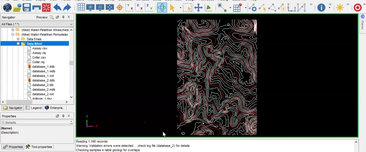
Stage 01 of the GEOVIA Surpac sequence: interpretation strings are reviewed across the available sections, preserving the boundaries used to construct the geological domain.
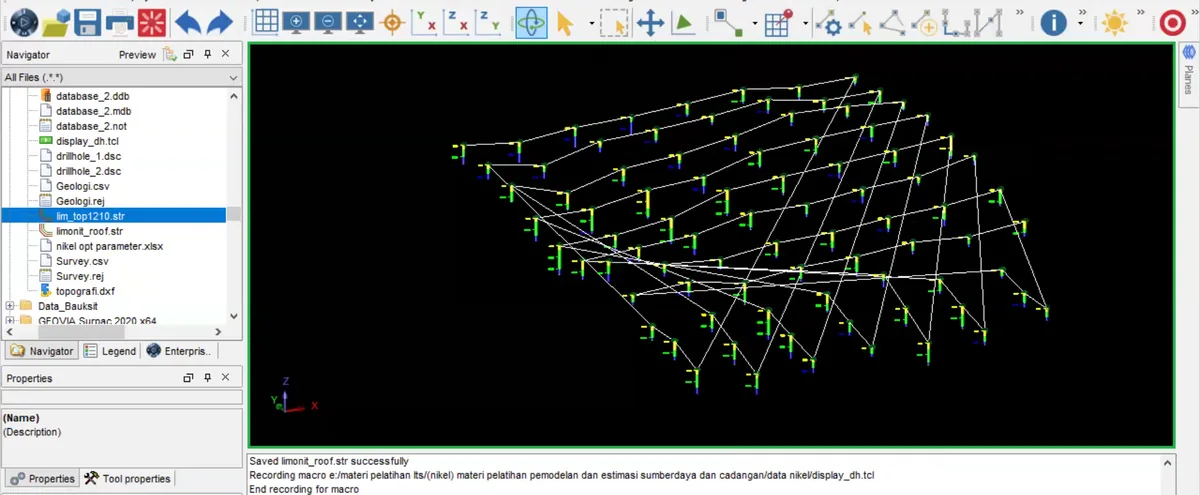
Stage 02 of the GEOVIA Surpac sequence: drillholes and their coded intervals are displayed in three dimensions to confirm collar positions, trace orientation and the spatial distribution of geological control.
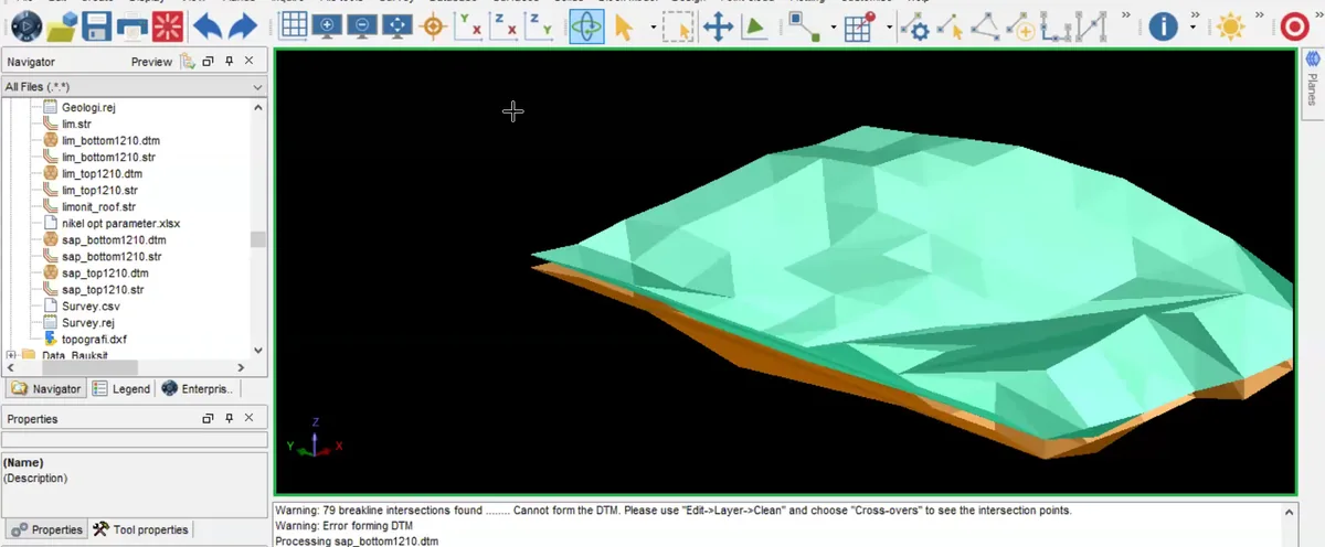
Stage 03 of the GEOVIA Surpac sequence: interpretation strings are reviewed across the available sections, preserving the boundaries used to construct the geological domain.
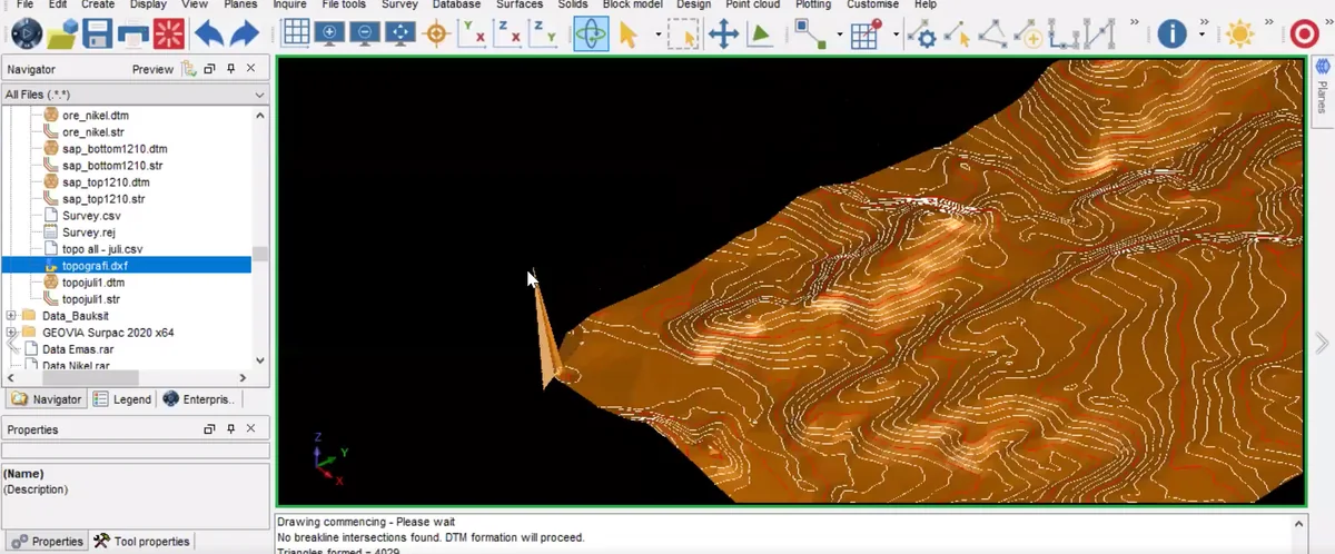
Stage 04 of the GEOVIA Surpac sequence: interpretation strings are reviewed across the available sections, preserving the boundaries used to construct the geological domain.
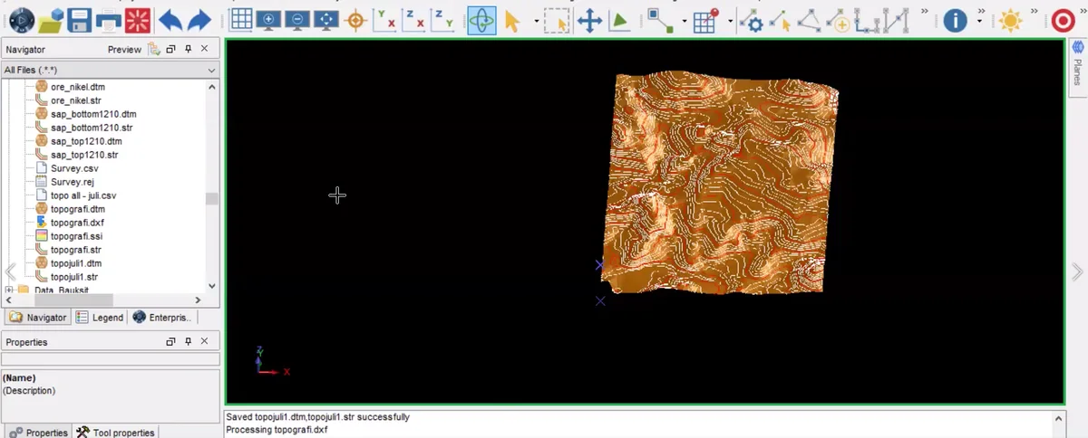
Stage 05 of the GEOVIA Surpac sequence: the GEOVIA Surpac project view displays the active geological objects at the wireframe construction stage.
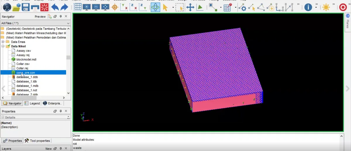
Stage 06 of the GEOVIA Surpac sequence: the interpreted boundary is converted into a triangulated surface and inspected for continuity, edge behaviour and local geometric artefacts.
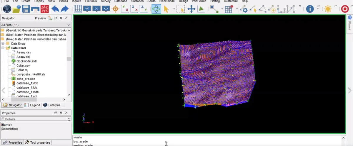
Stage 07 of the GEOVIA Surpac sequence: bounding surfaces are joined into a closed geological solid that represents the interpreted three-dimensional domain.
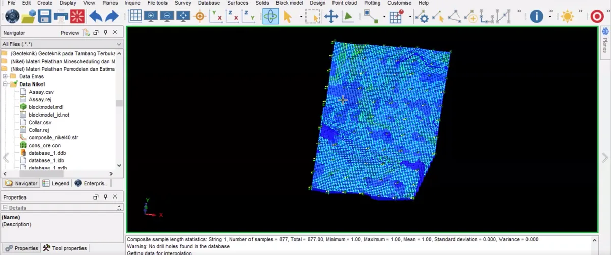
Stage 08 of the GEOVIA Surpac sequence: the geological interpretation is placed against the topographic surface to verify its position, extent and relationship with the ground surface.
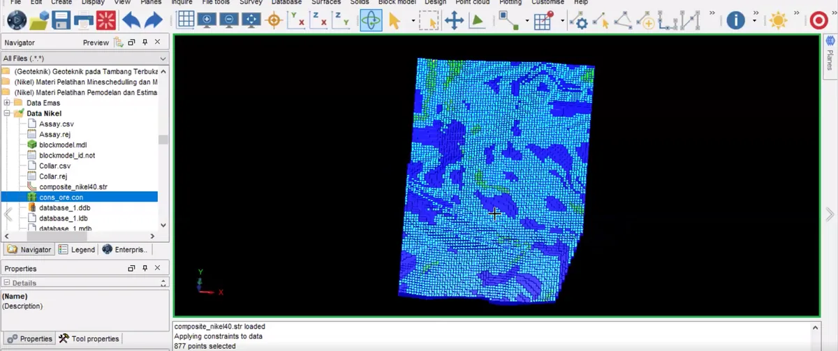
Stage 09 of the GEOVIA Surpac sequence: the interpreted surfaces, solids or model cells are isolated and compared to check continuity, boundary conformity and internal consistency.
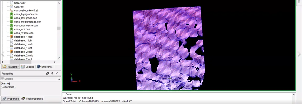
Stage 10 of the GEOVIA Surpac sequence: a regular three-dimensional cell framework is generated across the interpreted domain, providing the structure required to store geological or quantitative attributes.
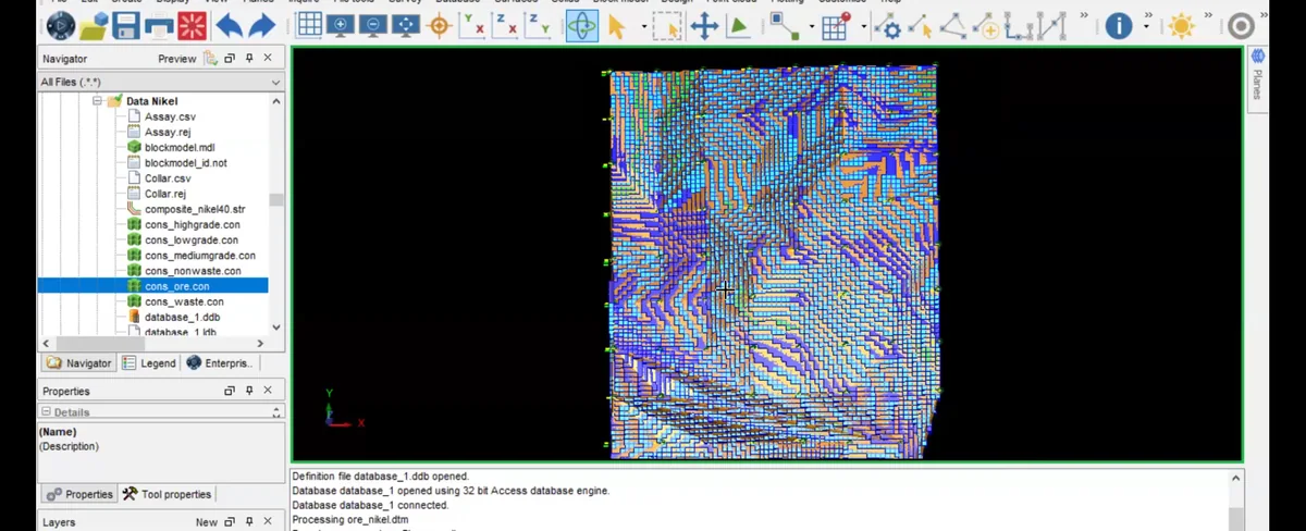
Stage 11 of the GEOVIA Surpac sequence: the model is coloured by an assigned attribute so that spatial changes and domain boundaries can be inspected directly.
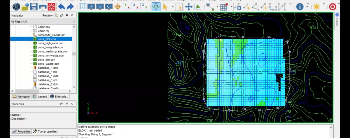
Stage 12 of the GEOVIA Surpac sequence: a sectional cut exposes the internal relationship between the model, interpreted boundaries and the available geological control.
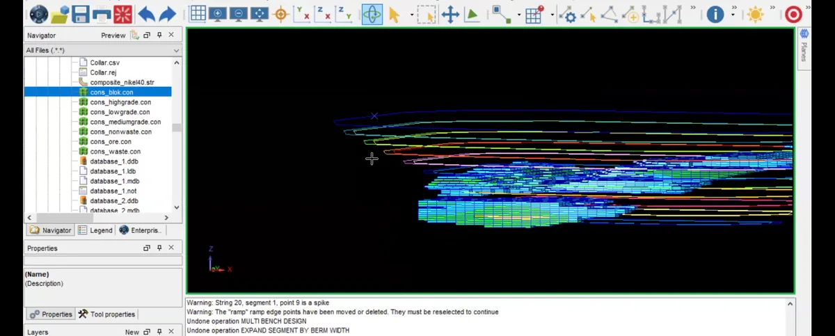
Stage 13 of the GEOVIA Surpac sequence: the interpreted surfaces, solids or model cells are isolated and compared to check continuity, boundary conformity and internal consistency.
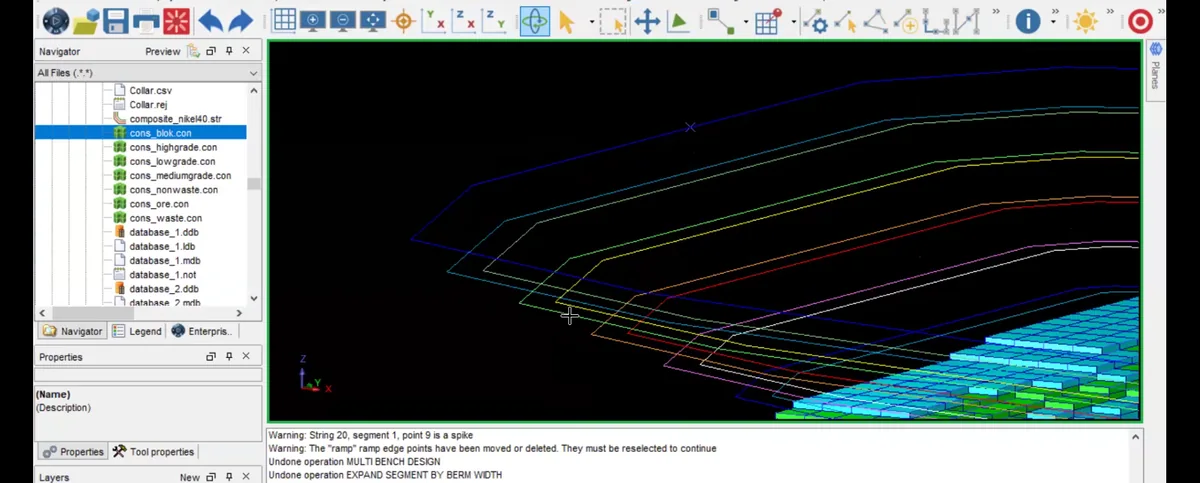
Stage 14 of the GEOVIA Surpac sequence: the interpreted surfaces, solids or model cells are isolated and compared to check continuity, boundary conformity and internal consistency.
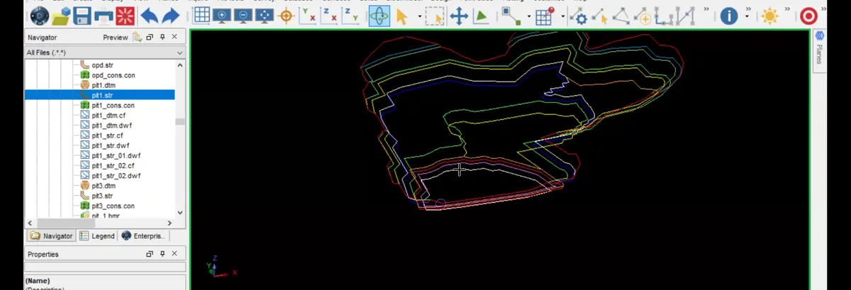
Stage 15 of the GEOVIA Surpac sequence: the interpreted surfaces, solids or model cells are isolated and compared to check continuity, boundary conformity and internal consistency.
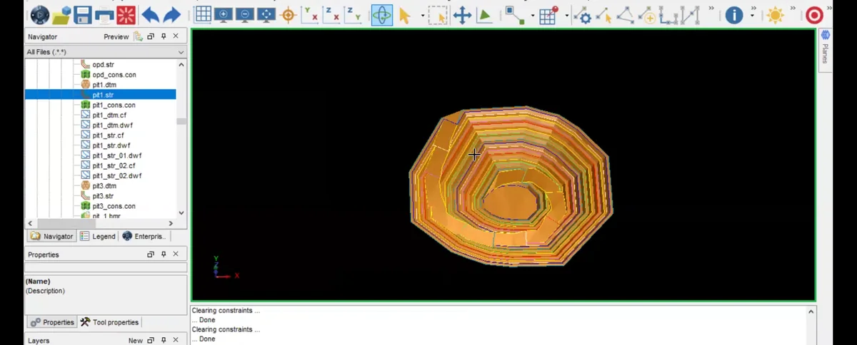
Stage 16 of the GEOVIA Surpac sequence: the principal model components are assembled in a final three-dimensional view for technical review and communication.
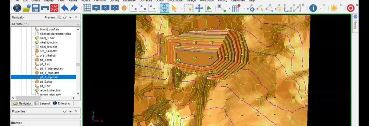
Stage 17 of the GEOVIA Surpac sequence: the principal model components are assembled in a final three-dimensional view for technical review and communication.
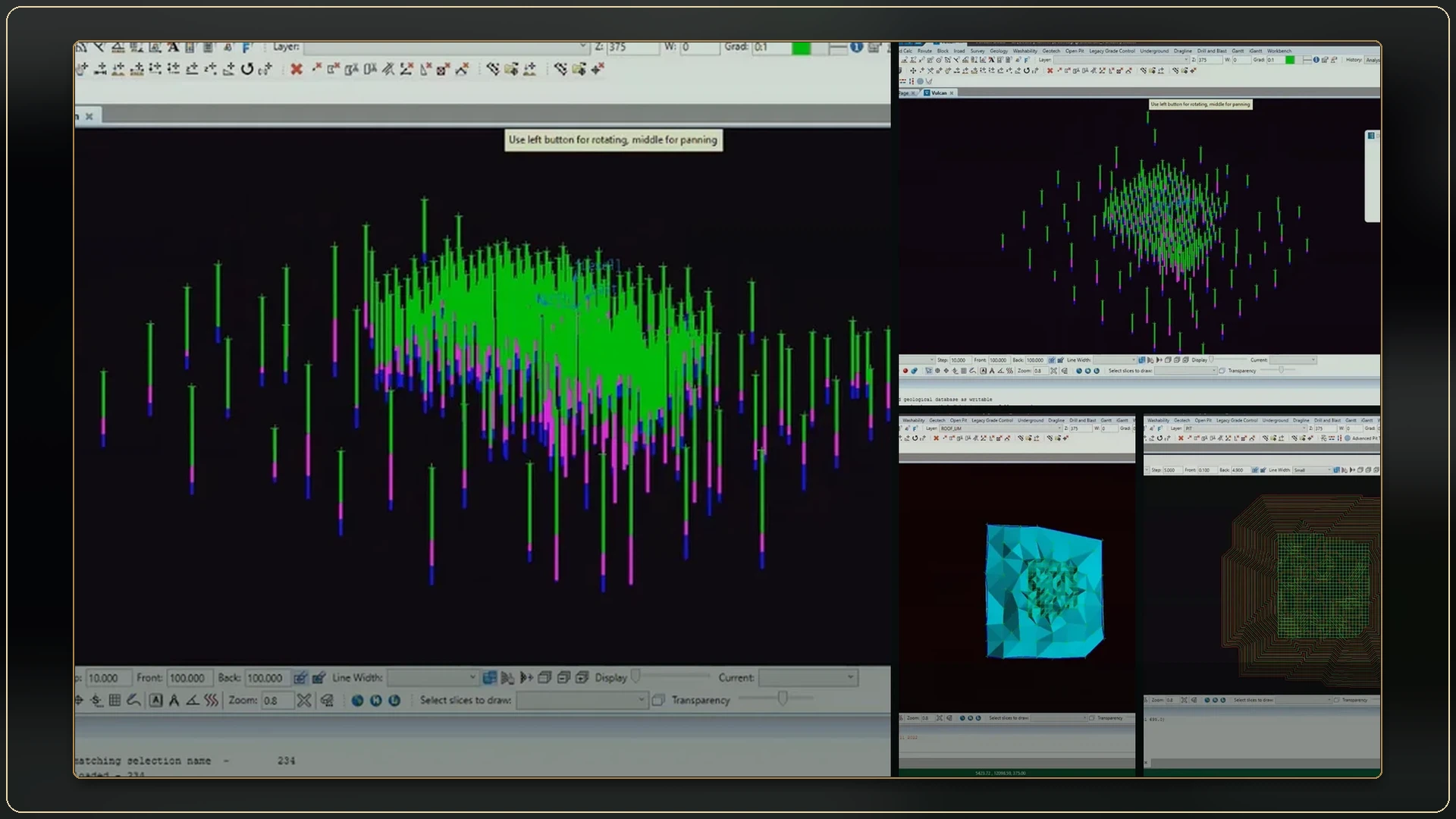
ALBUM
18 records
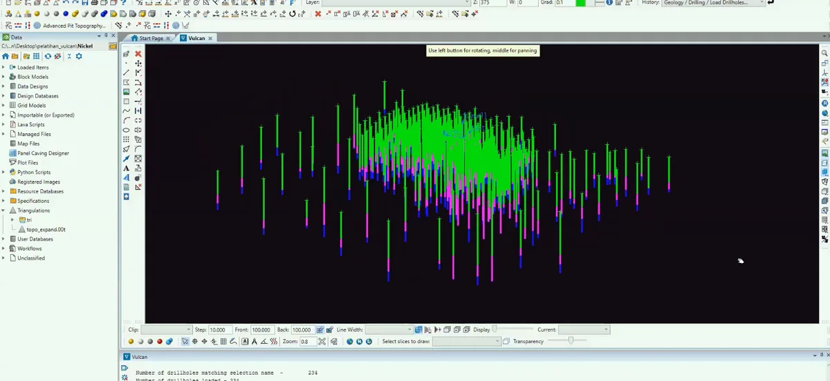
Stage 01 of the Maptek Vulcan sequence: the geological interpretation is placed against the topographic surface to verify its position, extent and relationship with the ground surface.
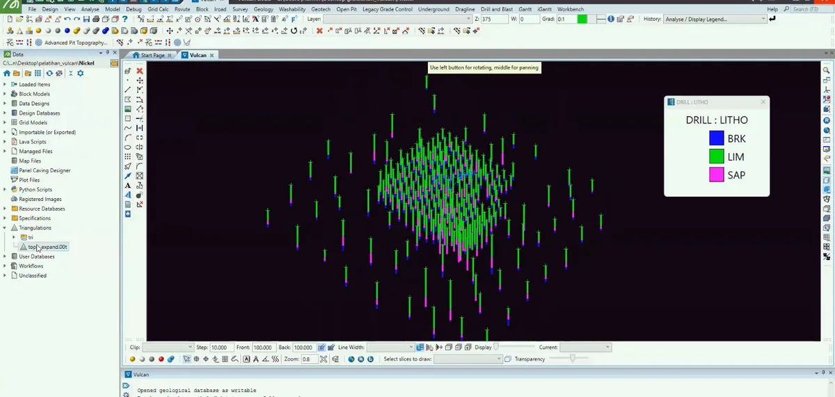
Stage 02 of the Maptek Vulcan sequence: the principal model components are assembled in a final three-dimensional view for technical review and communication.
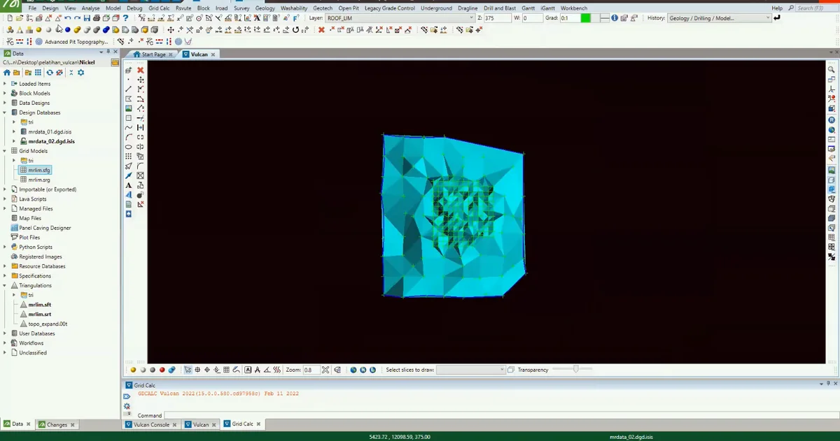
Stage 03 of the Maptek Vulcan sequence: drillholes and their coded intervals are displayed in three dimensions to confirm collar positions, trace orientation and the spatial distribution of geological control.
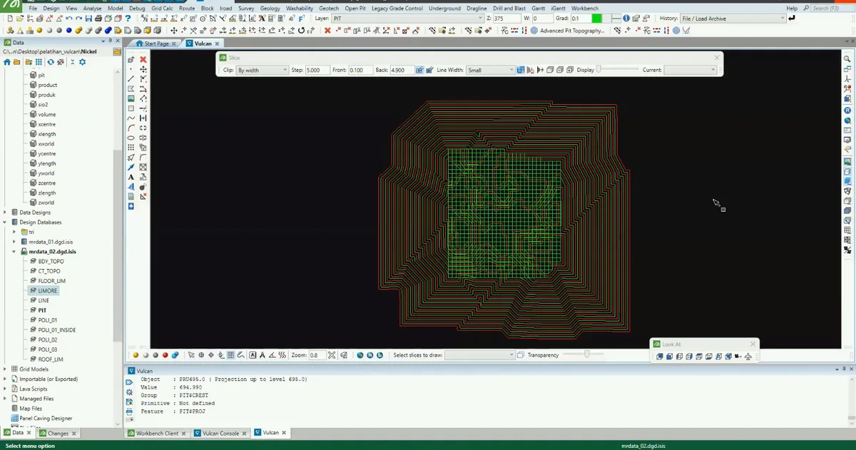
Stage 04 of the Maptek Vulcan sequence: interpretation strings are reviewed across the available sections, preserving the boundaries used to construct the geological domain.
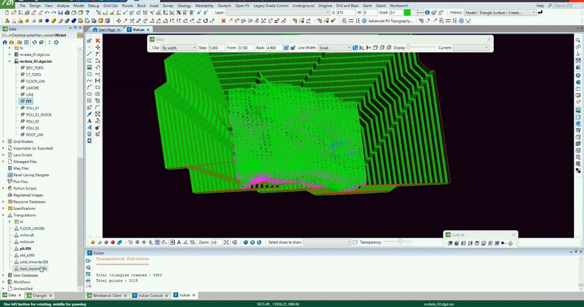
Stage 05 of the Maptek Vulcan sequence: the interpreted boundary is converted into a triangulated surface and inspected for continuity, edge behaviour and local geometric artefacts.
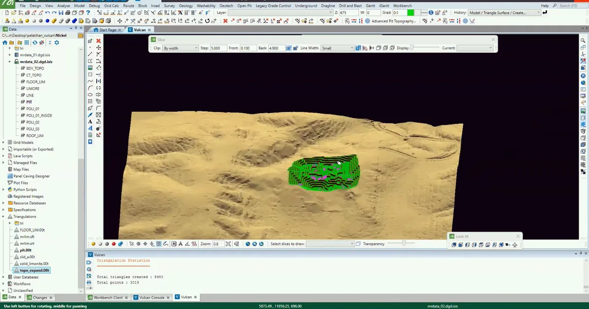
Stage 06 of the Maptek Vulcan sequence: the interpreted boundary is converted into a triangulated surface and inspected for continuity, edge behaviour and local geometric artefacts.
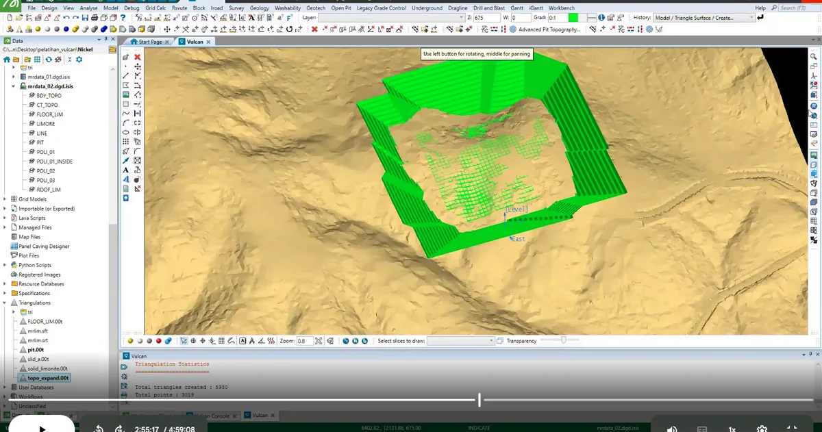
Stage 07 of the Maptek Vulcan sequence: bounding surfaces are joined into a closed geological solid that represents the interpreted three-dimensional domain.
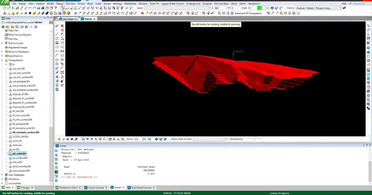
Stage 08 of the Maptek Vulcan sequence: the interpreted surfaces, solids or model cells are isolated and compared to check continuity, boundary conformity and internal consistency.
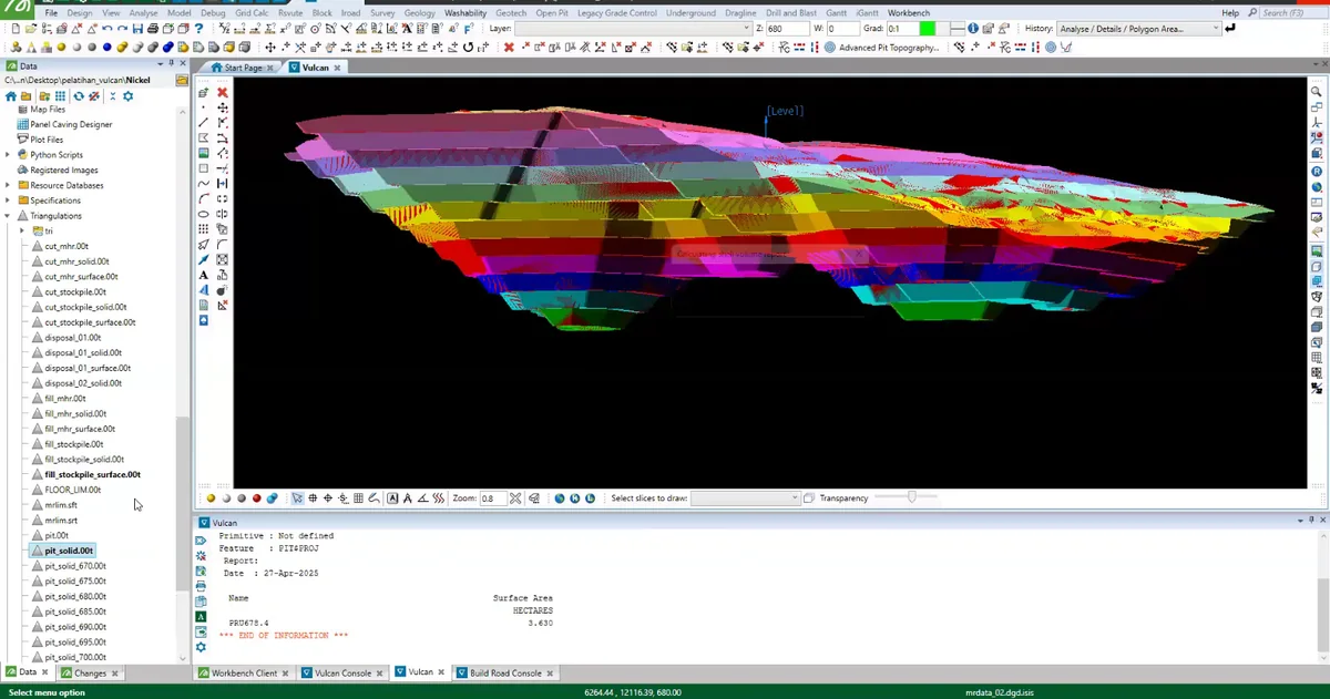
Stage 09 of the Maptek Vulcan sequence: a regular three-dimensional cell framework is generated across the interpreted domain, providing the structure required to store geological or quantitative attributes.
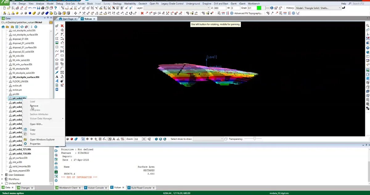
Stage 10 of the Maptek Vulcan sequence: the model is coloured by an assigned attribute so that spatial changes and domain boundaries can be inspected directly.
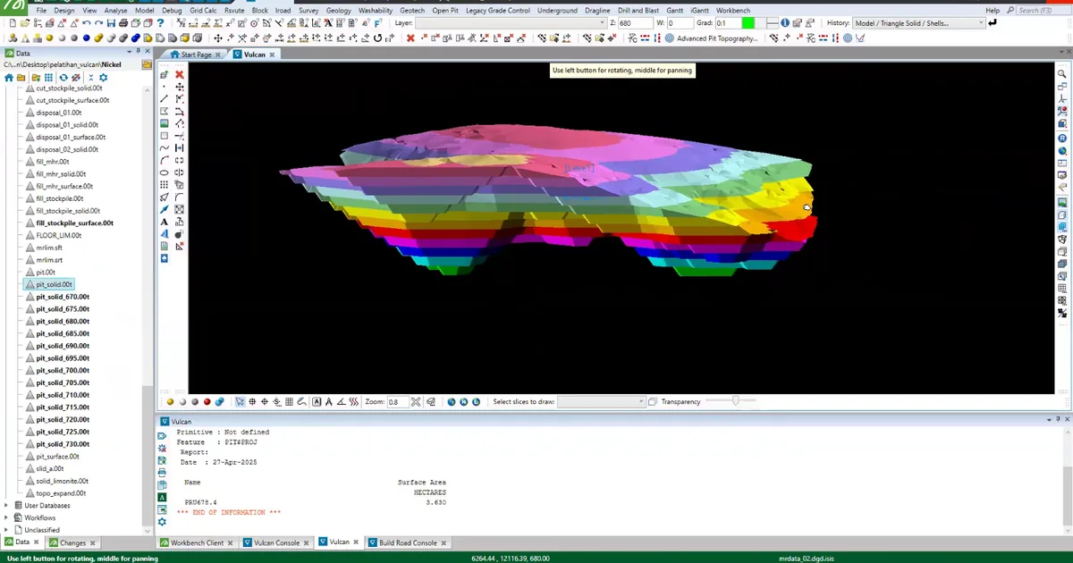
Stage 11 of the Maptek Vulcan sequence: the model is coloured by an assigned attribute so that spatial changes and domain boundaries can be inspected directly.
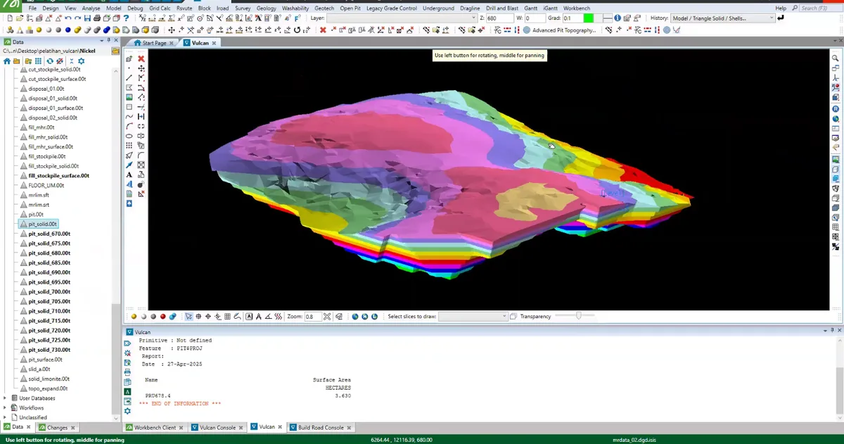
Stage 12 of the Maptek Vulcan sequence: a sectional cut exposes the internal relationship between the model, interpreted boundaries and the available geological control.
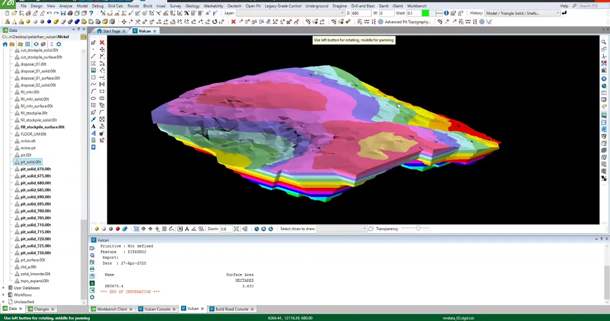
Stage 13 of the Maptek Vulcan sequence: the interpreted surfaces, solids or model cells are isolated and compared to check continuity, boundary conformity and internal consistency.
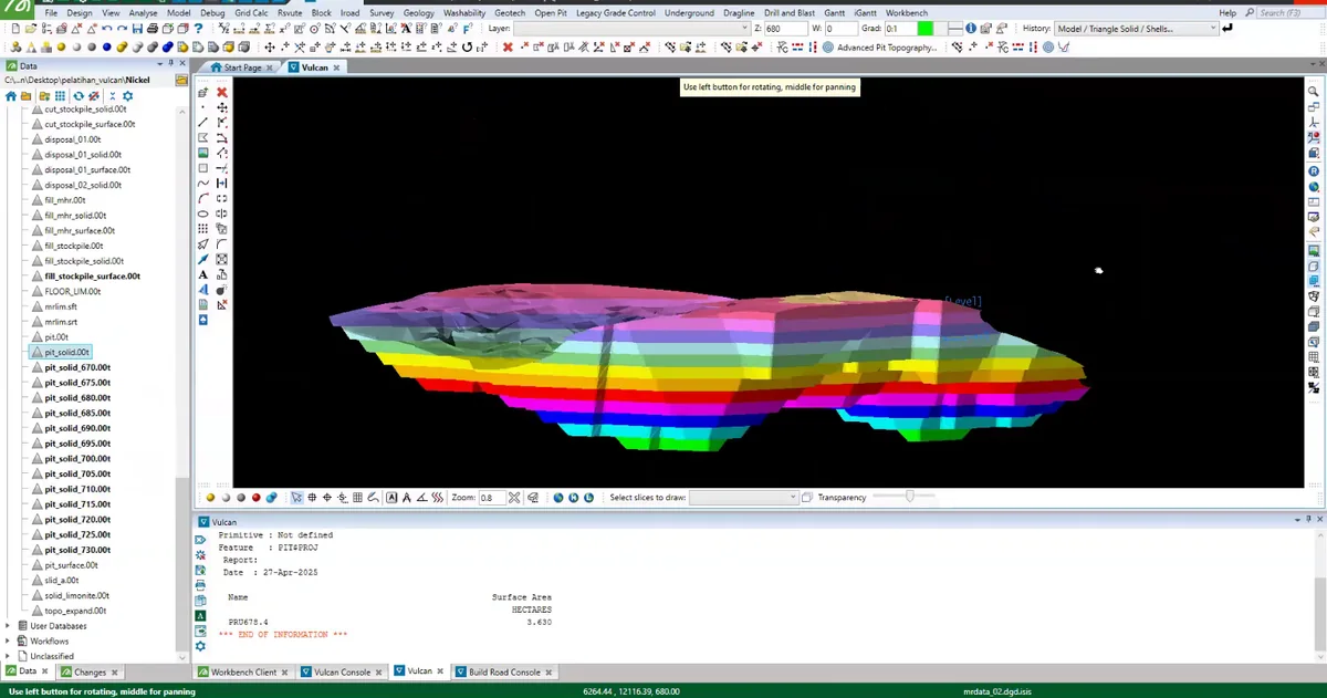
Stage 14 of the Maptek Vulcan sequence: the interpreted surfaces, solids or model cells are isolated and compared to check continuity, boundary conformity and internal consistency.
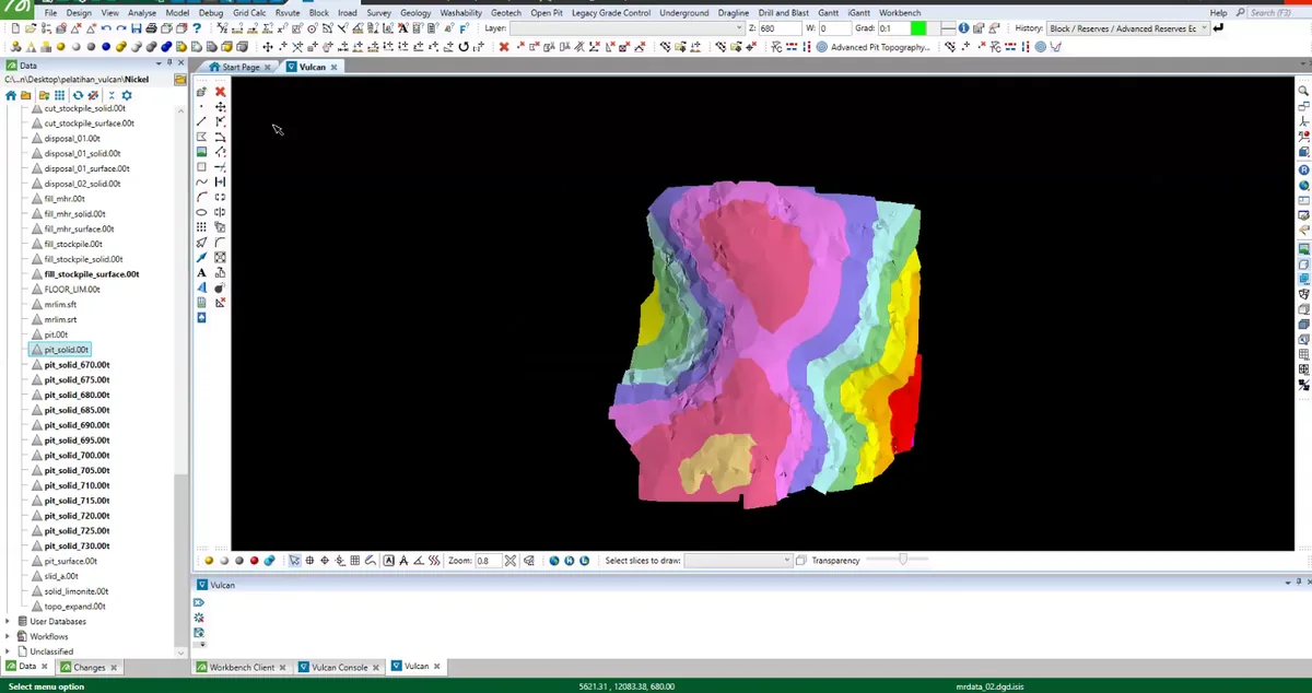
Stage 15 of the Maptek Vulcan sequence: the geological model is displayed with a design or volume boundary to examine the portion of the domain contained within the selected limit.
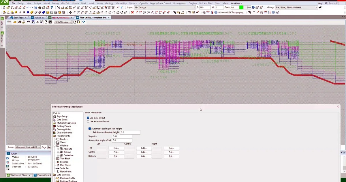
Stage 16 of the Maptek Vulcan sequence: the Maptek Vulcan project view displays the active geological objects at the integrated 3d scene stage.
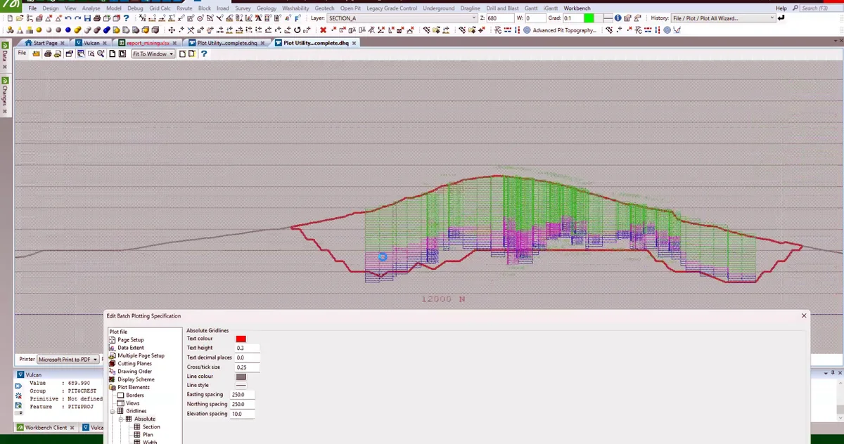
Stage 17 of the Maptek Vulcan sequence: the interpreted surfaces, solids or model cells are isolated and compared to check continuity, boundary conformity and internal consistency.
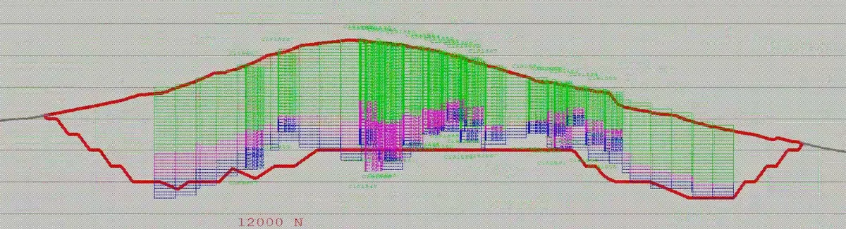
Stage 18 of the Maptek Vulcan sequence: the principal model components are assembled in a final three-dimensional view for technical review and communication.
ALBUM
4 records
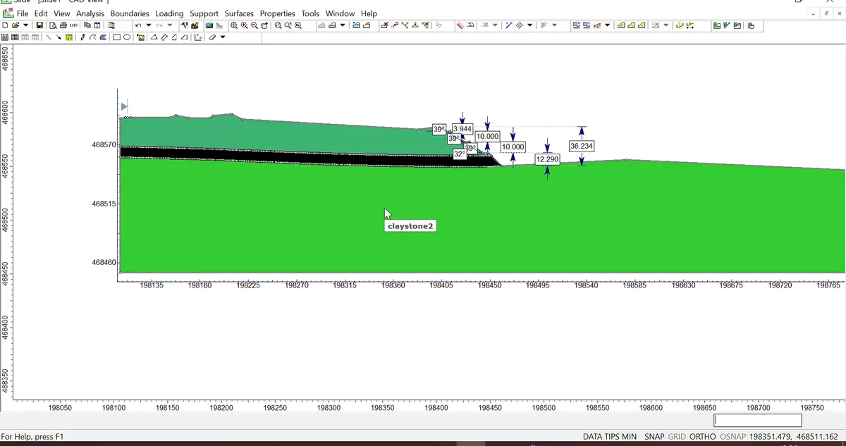
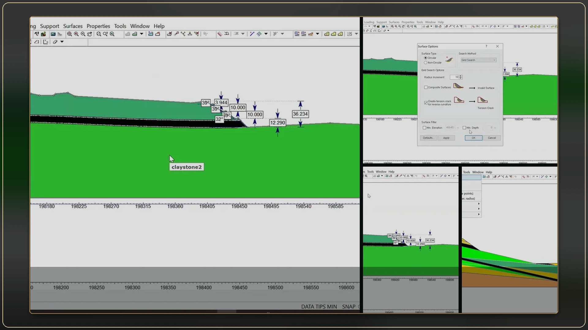
Stage 01 of the Rocscience Slide2 sequence: the section geometry and material units are drawn from the interpreted subsurface profile, preserving the principal layer boundaries and slope form.
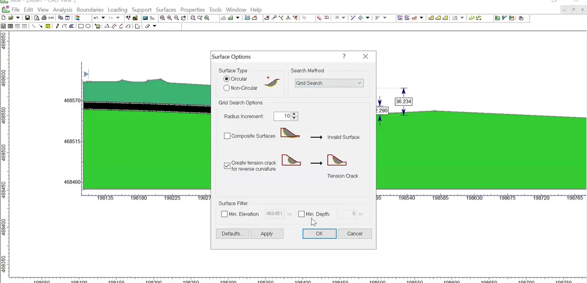
Stage 02 of the Rocscience Slide2 sequence: the search method and admissible slip-surface geometry are configured against the modelled slope section.
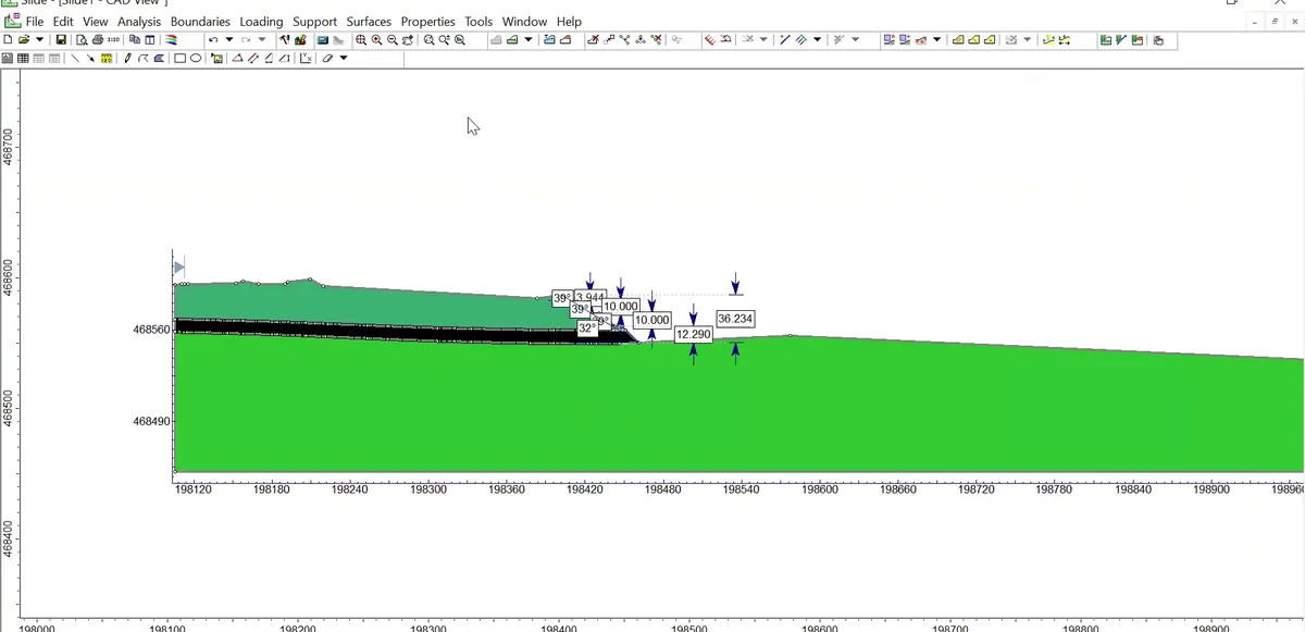
Stage 03 of the Rocscience Slide2 sequence: the completed slope model is submitted to the limit-equilibrium calculation after geometry, materials and search controls have been defined.
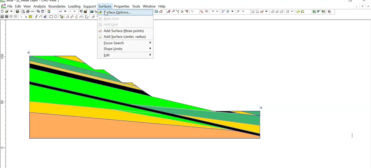
Stage 04 of the Rocscience Slide2 sequence: the interpreted stratigraphic section is reviewed with the analysis display to check the model geometry and the location of the calculated result.